Page 343 - Electromagnetics

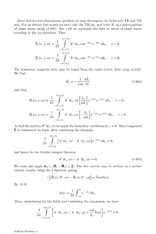
Since this is a two-dimensional problem we may decompose the fields into TE and TM
sets. For an electric line source we need only the TM set, and write E z as a superposition
of plane waves using (4.400). For y≷0 we represent the field in terms of plane waves
traveling in the ±y-direction. Thus
∞+ j
1
˜ + − jk x x − jk y y
E z (x, y,ω) = A (k x ,ω)e e dk x , y > 0,
2π
−∞+ j
∞+ j
1
˜ − − jk x x + jk y y
E z (x, y,ω) = A (k x ,ω)e e dk x , y < 0.
2π
−∞+ j
The transverse magnetic field may be found from the axial electric field using (4.212).
We find
˜
1 ∂E z
˜
H x =− (4.404)
jω ˜µ ∂y
and thus
∞+ j
1 k y
˜ + − jk x x − jk y y
H x (x, y,ω) = A (k x ,ω) e e dk x , y > 0,
2π ω ˜µ
−∞+ j
∞+ j
1 k y
˜ − − jk x x + jk y y
H x (x, y,ω) = A (k x ,ω) − e e dk x , y < 0.
2π ω ˜µ
−∞+ j
To find the spectra A (k x ,ω) we apply the boundary conditions at y = 0. Since tangential
±
˜
E is continuous we have, after combining the integrals,
∞+ j
1 − jk x x
+
A (k x ,ω) − A (k x ,ω) e dk x = 0,
−
2π
−∞+ j
and hence by the Fourier integral theorem
−
+
A (k x ,ω) − A (k x ,ω) = 0. (4.405)
˜
˜
˜
We must also apply ˆ n 12 × (H 1 − H 2 ) = J s . The line current may be written as a surface
current density using the δ-function, giving
˜
˜
˜

−
+
− H x (x, 0 ,ω) − H x (x, 0 ,ω) = I(ω)δ(x).
By (A.4)
1 ∞ − jk x x
δ(x) = e dk x .
2π
−∞
Then, substituting for the fields and combining the integrands, we have
∞+ j
1 ω ˜µ
+ − ˜ − jk x x
A (k x ,ω) + A (k x ,ω) + I(ω) e = 0,
2π k y
−∞+ j
© 2001 by CRC Press LLC