Page 382 - Electromagnetics

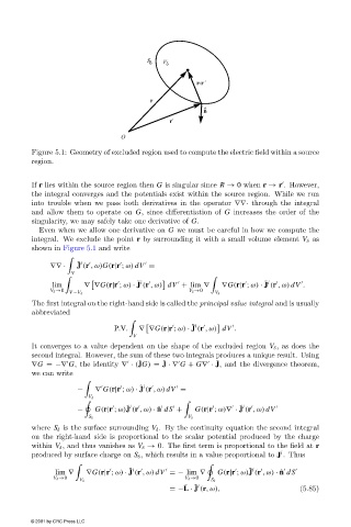
Figure 5.1: Geometry of excluded region used to compute the electric field within a source
region.

If r lies within the source region then G is singular since R → 0 when r → r . However,

the integral converges and the potentials exist within the source region. While we run
into trouble when we pass both derivatives in the operator ∇∇· through the integral
and allowthem to operate on G, since differentiation of G increases the order of the
singularity, we may safely take one derivative of G.
Even when we allow one derivative on G we must be careful in how we compute the
integral. We exclude the point r by surrounding it with a small volume element V δ as
shown in Figure 5.1 and write

˜ i
∇∇ · J (r ,ω)G(r|r ; ω) dV =
V

˜ i ˜ i
lim ∇ ∇G(r|r ; ω) · J (r ,ω) dV + lim ∇ ∇G(r|r ; ω) · J (r ,ω) dV .
V δ →0 V δ →0
V −V δ V δ
The first integral on the right-hand side is called the principal value integral and is usually
abbreviated

˜ i

P.V. ∇ ∇G(r|r ; ω) · J (r ,ω) dV .
V
It converges to a value dependent on the shape of the excluded region V δ , asdoesthe
second integral. However, the sum of these two integrals produces a unique result. Using
˜
˜
˜
∇G =−∇ G, the identity ∇ · (JG) = J ·∇ G + G∇ · J, and the divergence theorem,

we can write

˜ i
− ∇ G(r|r ; ω) · J (r ,ω) dV =
V δ

˜ i ˜ i
− G(r|r ; ω)J (r ,ω) · ˆ n dS + G(r|r ; ω)∇ · J (r ,ω) dV
S δ V δ
where S δ is the surface surrounding V δ . By the continuity equation the second integral
on the right-hand side is proportional to the scalar potential produced by the charge
within V δ , and thus vanishes as V δ → 0. The first term is proportional to the field at r
i
produced by surface charge on S δ , which results in a value proportional to J .Thus

˜ i ˜ i
lim ∇ ∇G(r|r ; ω) · J (r ,ω) dV =− lim ∇ G(r|r ; ω)J (r ,ω) · ˆ n dS
V δ →0 V δ →0
V δ S δ
¯ ˜ i
=−L · J (r,ω), (5.85)
© 2001 by CRC Press LLC