Page 384 - Electromagnetics

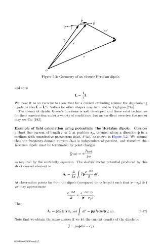
Figure 5.2: Geometry of an electric Hertzian dipole.

and thus
1
¯ ¯
L = I.
3
We leave it as an exercise to showthat for a cubical excluding volume the depolarizing
¯
¯
dyadic is also L = I/3. Values for other shapes may be found in Yaghjian [215].
The theory of dyadic Green’s functions is well developed and there exist techniques
for their construction under a variety of conditions. For an excellent overviewthe reader
may see Tai [192].
Example of field calculation using potentials: the Hertzian dipole. Consider
a short line current of length l λ at position r p , oriented along a direction ˆ p in a
c
medium with constitutive parameters ˜µ(ω), ˜ (ω), as shown in Figure 5.2. We assume
˜
that the frequency-domain current I(ω) is independent of position, and therefore this
Hertzian dipole must be terminated by point charges
˜ I(ω)
˜
Q(ω) =±
jω
as required by the continuity equation. The electric vector potential produced by this
short current element is
˜ µ e − jkR
˜ ˜
A e = I ˆ p dl .
4π R
At observation points far from the dipole (compared to its length) such that |r − r p | l
we may approximate
e − jkR e − jk|r−r p |
≈ .
R |r − r p |
Then

˜
˜
˜
A e = ˆ p ˜µIG(r|r p ; ω) dl = ˆ p ˜µIlG(r|r p ; ω). (5.87)

Note that we obtain the same answer if we let the current density of the dipole be
˜
J = jω˜ pδ(r − r p )

© 2001 by CRC Press LLC