Page 387 - Electromagnetics

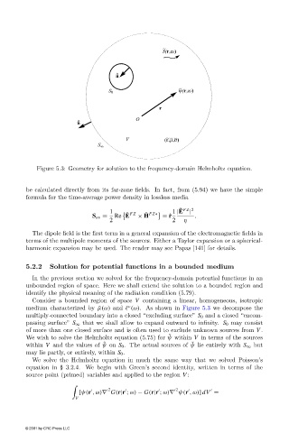
Figure 5.3: Geometry for solution to the frequency-domain Helmholtz equation.

be calculated directly from its far-zone fields. In fact, from (5.94) we have the simple
formula for the time-average power density in lossless media

ˇ FZ 2
1 1 |E |
ˇ FZ
ˇ FZ∗
S av = Re E × H = ˆ r .
2 2 η
The dipole field is the first term in a general expansion of the electromagnetic fields in
terms of the multipole moments of the sources. Either a Taylor expansion or a spherical-
harmonic expansion may be used. The reader may see Papas [141] for details.

5.2.2 Solution for potential functions in a bounded medium
In the previous section we solved for the frequency-domain potential functions in an
unbounded region of space. Here we shall extend the solution to a bounded region and
identify the physical meaning of the radiation condition (5.79).
Consider a bounded region of space V containing a linear, homogeneous, isotropic
c
medium characterized by ˜µ(ω) and ˜ (ω). As shown in Figure 5.3 we decompose the
multiply-connected boundary into a closed “excluding surface” S 0 and a closed “encom-
passing surface” S ∞ that we shall allow to expand outward to infinity. S 0 may consist
of more than one closed surface and is often used to exclude unknown sources from V .
˜
We wish to solve the Helmholtz equation (5.75) for ψ within V in terms of the sources
˜
˜
within V and the values of ψ on S 0 . The actual sources of ψ lie entirely with S ∞ but
may lie partly, or entirely, within S 0 .
We solve the Helmholtz equation in much the same way that we solved Poisson’s
equation in § 3.2.4. We begin with Green’s second identity, written in terms of the
source point (primed) variables and applied to the region V :

2 2
[ψ(r ,ω)∇ G(r|r ; ω) − G(r|r ; ω)∇ ψ(r ,ω)] dV =
V

© 2001 by CRC Press LLC