Page 421 - Electromagnetics

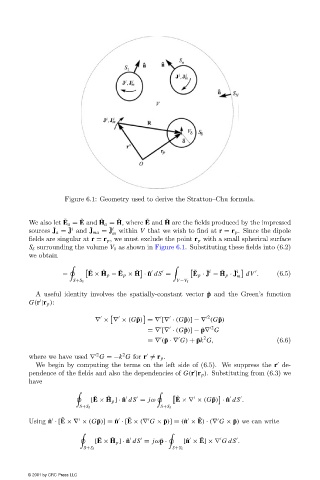
Figure 6.1: Geometry used to derive the Stratton–Chu formula.

˜
˜
˜
˜
˜
˜
We also let E a = E and H a = H, where E and H are the fields produced by the impressed
˜
˜
˜ i
˜ i
sources J a = J and J ma = J within V that we wish to find at r = r p . Since the dipole
m
fields are singular at r = r p , we must exclude the point r p with a small spherical surface
S δ surrounding the volume V δ as shown in Figure 6.1. Substituting these fields into (6.2)
we obtain

˜ ˜ ˜ ˜ ˜ ˜ i ˜ ˜ i

− E × H p − E p × H · ˆ n dS = E p · J − H p · J dV . (6.5)
m
S+S δ V −V δ
A useful identity involves the spatially-constant vector ˜ p and the Green’s function
G(r |r p ):

2
∇ × ∇ × (G ˜ p) =∇ [∇ · (G ˜ p)] −∇ (G ˜ p)

2

=∇ [∇ · (G ˜ p)] − ˜ p∇ G
2

=∇ (˜ p ·∇ G) + ˜ pk G, (6.6)
2
2
where we have used ∇ G =−k G for r = r p .

We begin by computing the terms on the left side of (6.5). We suppress the r de-

pendence of the fields and also the dependencies of G(r |r p ). Substituting from (6.3) we

have

˜
˜
˜

[E × H p ] · ˆ n dS = jω E ×∇ × (G ˜ p) · ˆ n dS .
S+S δ S+S δ
˜
˜
˜
Using ˆ n · [E ×∇ × (G ˜ p)] = ˆ n · [E × (∇ G × ˜ p)] = (ˆ n × E) · (∇ G × ˜ p) we can write

˜ ˜ ˜
[E × H p ] · ˆ n dS = jω˜ p · [ˆ n × E] ×∇ GdS .
S+S δ S+S δ
© 2001 by CRC Press LLC