Page 423 - Electromagnetics

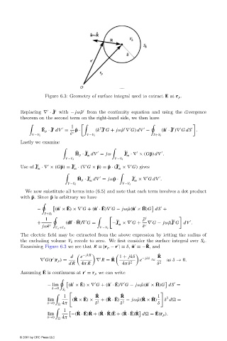
Figure 6.3: Geometry of surface integral used to extract E at r p .

i
˜ i

Replacing ∇ · J with − jω ˜ρ from the continuity equation and using the divergence
theorem on the second term on the right-hand side, we then have
1

˜ ˜ i 2 ˜ i i ˜ i
E p · J dV = ˜ p · (k J G + jω ˜ρ ∇ G) dV − (ˆ n · J )∇ GdS .
˜ c
V −V δ V −V δ S+S δ
Lastly we examine

˜ i
˜ i
˜
H p · J dV = jω J ·∇ × (G ˜ p) dV .

m m
V −V δ V −V δ
˜ i
˜ i
˜ i

Use of J ·∇ × (G ˜ p) = J · (∇ G × ˜ p) = ˜ p · (J ×∇ G) gives
m m m

˜ ˜ i ˜ i
H p · J dV = jω˜ p · J ×∇ GdV .
m
m
V −V δ V −V δ
We now substitute all terms into (6.5) and note that each term involves a dot product
with ˜ p. Since ˜ p is arbitrary we have

˜
˜ ˜
− (ˆ n × E) ×∇ G + (ˆ n · E)∇ G − jω ˜µ(ˆ n × H)G dS +
S+S δ
1 ˜ ρ i
˜ ˜ i ˜ i
+ c (dl · H)∇ G = −J ×∇ G + c ∇ G − jω ˜µJ G dV .
m
jω˜ ˜
a + b V −V δ
The electric field may be extracted from the above expression by letting the radius of
the excluding volume V δ recede to zero. We first consider the surface integral over S δ .
ˆ
Examining Figure 6.3 we see that R = |r p − r |= δ, ˆ n =−R, and

ˆ
d
e − jkR
1 + jkδ R
ˆ − jkδ
∇ G(r |r p ) = ∇ R = R e ≈ as δ → 0.
dR 4π R 4πδ 2 δ 2
˜
Assuming E is continuous at r = r p we can write

˜
˜
˜

− lim (ˆ n × E) ×∇ G + (ˆ n · E)∇ G − jω ˜µ(ˆ n × H)G dS =
δ→0
S δ

1 R R 1 2
ˆ ˆ
˜
ˆ
ˆ
ˆ
˜
˜
lim (R × E) × + (R · E) − jω ˜µ(R × H) δ d =
δ→0 4π δ 2 δ 2 δ

ˆ
˜
˜ ˆ
ˆ
˜ ˆ
ˆ
ˆ ˜
1
lim −(R · E)R + (R · R)E + (R · E)R d = E(r p ).
δ→0 4π
© 2001 by CRC Press LLC