Page 422 - Electromagnetics

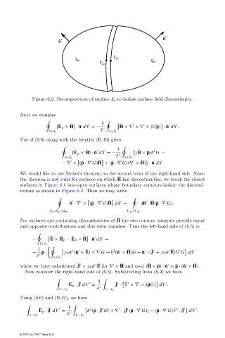
Figure 6.2: Decomposition of surface S n to isolate surface field discontinuity.

Next we examine
1
˜ ˜ ˜
[E p × H] · ˆ n dS =− H ×∇ ×∇ × (G ˜ p) · ˆ n dS .
˜ c
S+S δ S+S δ
Use of (6.6) along with the identity (B.43) gives
1

˜ ˜ ˜ 2
[E p × H] · ˆ n dS =− c (H × ˜ p)k G −
˜
S+S δ S+S δ
˜
˜

−∇ × (˜ p ·∇ G)H + (˜ p ·∇ G)(∇ × H) · ˆ n dS .
We would like to use Stokes’s theorem on the second term of the right-hand side. Since
˜
the theorem is not valid for surfaces on which H has discontinuities, we break the closed
surfaces in Figure 6.1 into open surfaces whose boundary contours isolate the disconti-
nuities as shown in Figure 6.2. Then we may write

˜ ˜
ˆ n ·∇ × (˜ p ·∇ G)H dS = dl · H(˜ p ·∇ G).
S n =S na +S nb na + nb
˜
For surfaces not containing discontinuities of H the two contour integrals provide equal
and opposite contributions and this term vanishes. Thus the left-hand side of (6.5) is

˜ ˜ ˜ ˜

− E × H p − E p × H · ˆ n dS =
S+S δ
1
c 2 c ˜
˜
˜
˜ i

− ˜ p · jω˜ (ˆ n × E) ×∇ G + k (ˆ n × H)G + ˆ n · (J + jω˜ E)∇ G dS
˜ c S+S δ
˜
˜
c ˜
˜
˜ i

where we have substituted J + jω˜ E for ∇ × H and used (H × ˜ p) · ˆ n = ˜ p · (ˆ n × H).
Now consider the right-hand side of (6.5). Substituting from (6.4) we have
1

˜ ˜ i ˜ i
E p · J dV = J · ∇ ×∇ × (˜ pG) dV .
˜ c
V −V δ V −V δ
Using (6.6) and (B.42), we have

1
˜ ˜ i 2 ˜ i ˜ i ˜ i
E p · J dV = k (˜ p · J )G +∇ · [J (˜ p ·∇ G)] − (˜ p ·∇ G)∇ · J dV .
˜ c
V −V δ V −V δ
© 2001 by CRC Press LLC