Page 460 - Electromagnetics

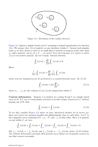
Figure A.1: Derivation of the residue theorem.

Figure A.1 depicts a simple closed curve C enclosing n isolated singularities of a function
f (z). We assume that f (z) is analytic on and elsewhere within C. Around each singular
point z k we have drawn a circle C k so small that it encloses no singular point other than
z k ; taken together, the C k (k = 1,..., n) and C form the boundary of a region in which
f (z) is everywhere analytic. By the Cauchy–Goursat theorem

n

f (z) dz + f (z) dz = 0.
C k=1 C k
Hence
n

1 1
f (z) dz = f (z) dz,
2π j C k=1 2π j C k
where now the integrations are all performed in a counterclockwise sense. By (A.12)
n

f (z) dz = 2π j r k (A.14)
C k=1
where r 1 ,...,r n are the residues of f (z) at the singularities within C.

Contour deformation. Suppose f is analytic in a region D and is a simple closed
curve in D.If can be continuously deformed to another simple closed curve without

passing out of D, then

f (z) dz = f (z) dz. (A.15)

To see this, consider Figure A.2 where we have introduced another set of curves ±γ ;
these new curves are assumed parallel and infinitesimally close to each other. Let C be

the composite curve consisting of , +γ , − , and −γ , in that order. Since f is analytic
on and within C, we have

f (z) dz = f (z) dz + f (z) dz + f (z) dz + f (z) dz = 0.
C +γ − −γ

But f (z) dz =− f (z) dz and f (z) dz =− f (z) dz, hence (A.15) follows.
− −γ +γ
The contour deformation principle often permits us to replace an integration contour by
one that is more convenient.

© 2001 by CRC Press LLC