Page 462 - Electromagnetics

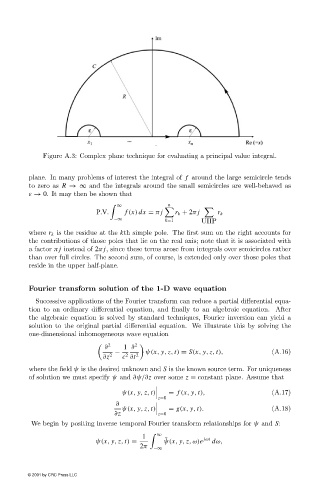
Figure A.3: Complex plane technique for evaluating a principal value integral.

plane. In many problems of interest the integral of f around the large semicircle tends
to zero as R →∞ and the integrals around the small semicircles are well-behaved as
ε → 0. It may then be shown that

n

∞

P.V. f (x) dx = π j r k + 2π j r k
−∞ k=1 UHP
where r k is the residue at the kth simple pole. The first sum on the right accounts for
the contributions of those poles that lie on the real axis; note that it is associated with
a factor π j instead of 2π j, since these terms arose from integrals over semicircles rather
than over full circles. The second sum, of course, is extended only over those poles that
reside in the upper half-plane.

Fourier transform solution of the 1-D wave equation
Successive applications of the Fourier transform can reduce a partial differential equa-
tion to an ordinary differential equation, and finally to an algebraic equation. After
the algebraic equation is solved by standard techniques, Fourier inversion can yield a
solution to the original partial differential equation. We illustrate this by solving the
one-dimensional inhomogeneous wave equation
∂ 1 ∂
2 2
− ψ(x, y, z, t) = S(x, y, z, t), (A.16)
2
∂z 2 c ∂t 2
where the field ψ is the desired unknown and S is the known source term. For uniqueness
of solution we must specify ψ and ∂ψ/∂z over some z = constant plane. Assume that

= f (x, y, t), (A.17)

ψ(x, y, z, t)
z=0
∂
= g(x, y, t). (A.18)

∂z z=0
ψ(x, y, z, t)
We begin by positing inverse temporal Fourier transform relationships for ψ and S:
1 ∞ jωt
˜
ψ(x, y, z, t) = ψ(x, y, z,ω)e dω,
2π
−∞
© 2001 by CRC Press LLC