Page 464 - Electromagnetics

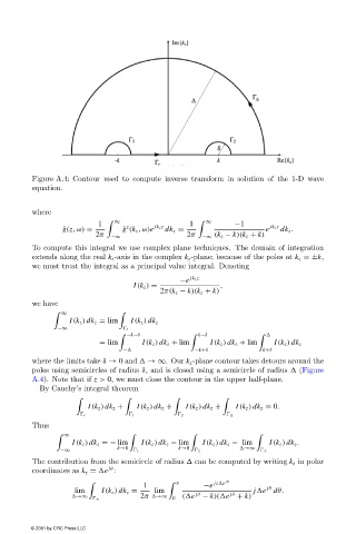
Figure A.4: Contour used to compute inverse transform in solution of the 1-D wave
equation.

where
1 ∞ z jk z z 1 ∞ −1 jk z z
˜ g(z,ω) = ˜ g (k z ,ω)e dk z = e dk z .
2π 2π −∞ (k z − k)(k z + k)
−∞
To compute this integral we use complex plane techniques. The domain of integration
extends along the real k z -axis in the complex k z -plane; because of the poles at k z =±k,
we must treat the integral as a principal value integral. Denoting
−e jk z z
I (k z ) = ,
2π(k z − k)(k z + k)
we have
∞

I (k z ) dk z = lim I (k z ) dk z
−∞ r
−k−δ k−δ
= lim I (k z ) dk z + lim I (k z ) dk z + lim I (k z ) dk z
− −k+δ k+δ
where the limits take δ → 0 and →∞. Our k z -plane contour takes detours around the
poles using semicircles of radius δ, and is closed using a semicircle of radius (Figure
A.4). Note that if z > 0, we must close the contour in the upper half-plane.
By Cauchy’s integral theorem

I (k z ) dk z + I (k z ) dk z + I (k z ) dk z + I (k z ) dk z = 0.
r 1 2
Thus
∞

I (k z ) dk z =− lim I (k z ) dk z − lim I (k z ) dk z − lim I (k z ) dk z .
δ→0 δ→0 →∞
−∞ 1 2
The contribution from the semicircle of radius can be computed by writing k z in polar
jθ
coordinates as k z = e :
1 −e jθ
π jz e jθ
lim I (k z ) dk z = lim j e dθ.
→∞ 2π →∞ 0 ( e jθ − k)( e jθ + k)

© 2001 by CRC Press LLC