Page 193 -

∆ te jω( t ∆ ) + 1
H = (6.106)
T jω( t ∆ )
2 e − 1

H = t ∆ e jω( t ∆ )/2 (6.107)
MP jω( t ∆ )
e − 1
∆ te ( j (ω t ∆ ) ++ e j − ω ( t ∆ ) )
4
H = (6.108)
S j (ω t ∆ ) j − ω ( t ∆ )
3 e − e
The measures of accuracy of the integration scheme are the ratios of these
Transfer Functions to that of the exact expression. These are given, respec-
tively, by:

(ω∆ t/ )2
R = cos(ω∆ t/ ) 2 (6.109)
T sin(ω∆ t/ ) 2

(ω∆ t/ )2
R = (6.110)
MP sin(ω∆ t/ )2

 ω∆ t cos( ω∆ t + 2)
R =   (6.111)
S  3  sin( ω∆ t)

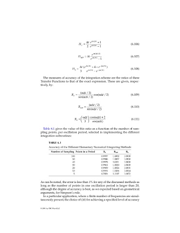
Table 6.1 gives the value of this ratio as a function of the number of sam-
pling points, per oscillation period, selected in implementing the different
integration subroutines:

TABLE 6.1
Accuracy of the Different Elementary Numerical Integrating Methods
Number of Sampling Points in a Period R T R MP R S
100 0.9997 1.0002 1.0000
50 0.9986 1.0007 1.0000
40 0.9978 1.0011 1.0000
30 0.9961 1.0020 1.0000
20 0.9909 1.0046 1.0001
10 0.9591 1.0206 1.0014
5 0.7854 1.1107 1.0472

As can be noted, the error is less than 1% for any of the discussed methods as
long as the number of points in one oscillation period is larger than 20,
although the degree of accuracy is best, as we expected based on geometrical
arguments, for Simpson’s rule.
In a particular application, where a finite number of frequencies are simul-
taneously present, the choice of (∆t) for achieving a specified level of accuracy

© 2001 by CRC Press LLC