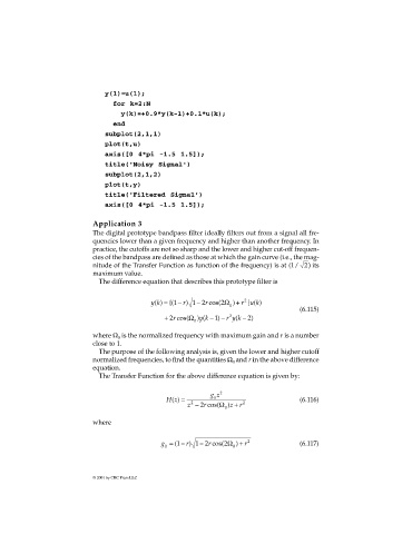
Page 196 -

y(1)=u(1);
for k=2:N
y(k)=+0.9*y(k-1)+0.1*u(k);
end
subplot(2,1,1)
plot(t,u)
axis([0 4*pi -1.5 1.5]);
title('Noisy Signal')
subplot(2,1,2)
plot(t,y)
title('Filtered Signal')
axis([0 4*pi -1.5 1.5]);

Application 3
The digital prototype bandpass filter ideally filters out from a signal all fre-
quencies lower than a given frequency and higher than another frequency. In
practice, the cutoffs are not so sharp and the lower and higher cut-off frequen-
cies of the bandpass are defined as those at which the gain curve (i.e., the mag-
nitude of the Transfer Function as function of the frequency) is at (/1 ) 2 its
maximum value.
The difference equation that describes this prototype filter is

−
yk( ) = {( −1 r) 1 2 r cos(2Ω ) + r u k} ( )
2
0
(6.115)
2
+ 2 r cos(Ω ) y k( − 1 ) − r y k( − 2 )
0
where Ω is the normalized frequency with maximum gain and r is a number
0
close to 1.
The purpose of the following analysis is, given the lower and higher cutoff
normalized frequencies, to find the quantities Ω and r in the above difference
0
equation.
The Transfer Function for the above difference equation is given by:

gz 2
Hz() = 0 (6.116)
2
z − 2 r cos(Ω ) z r+ 2
0
where

g = ( 1− r 1 2−) r cos( 2Ω ) + r 2 (6.117)
0 0

© 2001 by CRC Press LLC