Page 68 -

define the iterated quantities by two indices: the order of the function and the
value of the argument of the function.
In many electrical engineering problems, it is convenient to use a class of
polynomials called the orthogonal polynomials. For example, in filter design,
the set of Chebyshev polynomials are of particular interest.
The Chebyshev polynomials can be defined through recursion relations,
which are similar to difference equations and relate the value of a polynomial
of a certain order at a particular point to the values of the polynomials of
lower orders at the same point. These are defined through the following
recursion relation:

T (x) = 2xT (x) – T (x) (2.46)
k–2
k
k–1
Now, instead of giving two values for the initial conditions as we would have
in difference equations, we need to give the explicit functions for two of the
lower-order polynomials. For example, the first- and second-order Cheby-
shev polynomials are

T (x) = x (2.47)
1
2
T (x) = 2x – 1 (2.48)
2
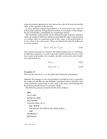
Example 2.7
Plot over the interval 0 ≤ x ≤ 1, the fifth-order Chebyshev polynomial.

Solution: The strategy to solve this problem is to build an array to represent
the x-interval, and then use the difference equation routine to find the value
of the Chebyshev polynomial at each value of the array, remembering that
the indexing should always be a positive integer.
The following program implements the above strategy:

N=5;
x1=1:101;
x=(x1-1)/100;
T(1,x1)=x;
T(2,x1)=2*x.^2-1;
for k=3:N
T(k,x1)=2.*x.*T(k-1,x1)-T(k-2,x1);
end
y=T(N,x1);
plot(x,y)

© 2001 by CRC Press LLC