Page 66 -

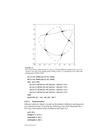
FIGURE 2.4
Plot of two Hénon orbits having the same a = 0.25 but different starting points. (o) corre-
sponds to the orbit with starting point (0.5696, 0.1622), (x) corresponds to the orbit with
starting point (0.5650, 0.1650).

x1(1)=0.5696;y1(1)=0.1622;
x2(1)=0.5650;y2(1)=0.1650;
for n=1:120
x1(n+1)=a*x1(n)-b*(y1(n)-(x1(n))^2);
y1(n+1)=b*x1(n)+a*(y1(n)-(x1(n))^2);
x2(n+1)=a*x2(n)-b*(y2(n)-(x2(n))^2);
y2(n+1)=b*x2(n)+a*(y2(n)-(x2(n))^2);
end
plot(x1,y1,'ro',x2,y2,'bx')

2.8.2.1 Demonstration
Different orbits for Hénon’s model can be plotted if different starting points
are randomly chosen. Executing the following script M-file illustrates the a =
0.24 case, with random initial conditions. See Figure 2.5.

a=0.24;
b=sqrt(1-a^2);
rx=rand(1,40);
ry=rand(1,40);

© 2001 by CRC Press LLC