Page 61 -

above model is used to simulate a population growth model. Specifically, in
an ecological or growth process, the normalized measure y(k + 1) of the next
generation of a specie (the number of animals, for example) is a linear func-
tion of the present measure y(k); that is,

y(k + 1) = ry(k) (2.41)

where r is the growth parameter. If unchecked, the growth of the specie fol-
lows a geometric series, which for r > 1 grows to infinity. But growth is often
limited by finite resources. In other words, the larger y(k), the smaller the
growth factor. The simplest way to model this decline in the growth factor is
to replace r by r(1 – y(k)), so that as y(k) approaches the theoretical limit (1 in
this case), the effective growth factor goes to zero. The difference equation
goes to:
y(k + 1) = r(1 – y(k))y(k) (2.42)

which is the standard form for the logistic equation.
In the next series of exercises, we explore the solution of Eq. (2.42) as we
vary the value of r. We find that qualitatively different classes of solutions
may appear for different values of r.
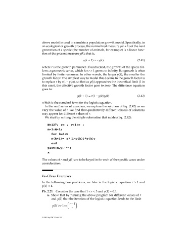
We start by writing the simple subroutine that models Eq. (2.42):

N=127; r= ; y(1)= ;
m=1:N+1;
for k=1:N
y(k+1)= r*(1-y(k))*y(k);
end
plot(m,y,'*')
x
The values of r and y(1) are to be keyed in for each of the specific cases under
consideration.

In-Class Exercises

In the following two problems, we take in the logistic equation r > 1 and
y(1) < 1.

Pb. 2.21 Consider the case that 1 < r < 3 and y(1) = 0.5.
a. Show that by running the above program for different values of r
and y(1) that the iteration of the logistic equation leads to the limit

(
yN >> 1 ) =  r −  1 .
 r 

© 2001 by CRC Press LLC