Page 20 - Elements of Distribution Theory

P1: JZP
052184472Xc01 CUNY148/Severini May 24, 2005 17:52

6 Properties of Probability Distributions

vector X is of the form
 
X 1
 X 2 
X =  . 
.
 . 
X d
where X 1 , X 2 ,..., X d are real-valued random variables.
For convenience, when writing a d-dimensional random vector in the text, we will write
T
X = (X 1 ,..., X d ) rather than X = (X 1 ,..., X d ) . Also, if X and Y are both random
vectors, the random vector formed by combining X and Y will be written as (X, Y), rather
T
T T
than the more correct, but more cumbersome, (X , Y ) .We will often consider random
vectors of the form (X, Y) with range X × Y;a statement of this form should be taken to
mean that X takes values in X and Y takes values in Y.
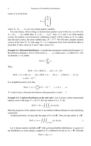
Example1.4 (Binomialdistribution). ConsidertheexperimentconsideredinExample1.2.
Recall that an element ω of is of the form (x 1 ,..., x n ) where each x j is either 0 or 1. For
an element ω ∈ , define
n

X(ω) = x j .
j=1
Then
n
Pr(X = 0) = P((0, 0,..., 0)) = (1 − θ) ,
Pr(X = 1) = P((1, 0,..., 0)) + P((0, 1, 0,..., 0)) +· · · + P((0, 0,..., 0, 1))
= nθ(1 − θ) n−1 .

It is straightforward to show that

n x n−x
Pr(X = x) = θ (1 − θ) , x = 0, 1,..., n;
x
X is said to have a binomial distribution with parameters n and θ.

Example 1.5 (Uniform distribution on the unit cube). Let X denote a three-dimensional
3
random vector with range X = (0, 1) .For any subset of A ∈ X, let

Pr(X ∈ A) = dt 1 dt 2 dt 3 .
A
Here the properties of the random vector X are defined without reference to any underlying
experiment.
3
3
As discussed above, we may take the range of X to be R . Then, for any subset A ∈ R ,

Pr(X ∈ A) = dt 1 dt 2 dt 3 .
A∩(0,1) 3

d
Let X denote random variable on R with a given probability distribution. A support of
d
the distribution, or, more simply, a support of X,is defined to be any set X 0 ⊂ R such that
Pr(X ∈ X 0 ) = 1.