Page 23 - Elements of Distribution Theory

P1: JZP
052184472Xc01 CUNY148/Severini May 24, 2005 17:52

1.4 Distribution Functions 9

F (x)

− −
x
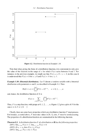
Figure 1.2. Distribution function in Example 1.10.

Note that when giving the form of a distribution function, it is convenient to only give
the value of the function in the range of x for which F(x)varies between 0 and 1. For
instance, in the previous example, we might say that F(x) = x,0 < x < 1; in this case it
is understood that F(x) = 0 for x ≤ 0 and F(x) = 1 for x ≥ 1.

Example 1.10 (Binomial distribution). Let X denote a random variable with a binomial
distribution with parameters n and θ,as described in Example 1.4. Then

n x n−x
Pr(X = x) = θ (1 − θ) , x = 0, 1,..., n
x
and, hence, the distribution function of X is

n j n− j
F(x) = θ (1 − θ) .
j
j=0,1,...; j≤x
Thus, F is a step function, with jumps at 0, 1, 2,..., n; Figure 1.2 gives a plot of F for the
case n = 2, θ = 1/4.

Clearly, there are some basic properties which any distribution function F must possess.
For instance, as noted above, F must take values in [0, 1]; also, F must be nondecreasing.
The properties of a distribution function are summarized in the following theorem.

Theorem 1.2. A distribution function F of a distribution on R has the following properties:
(DF1) lim x→∞ F(x) = 1; lim x→−∞ F(x) = 0
(DF2) If x 1 < x 2 then F(x 1 ) ≤ F(x 2 )
(DF3) lim h→0 F(x + h) = F(x)
+