Page 217 - Elements of Distribution Theory

P1: JZX
052184472Xc07 CUNY148/Severini May 24, 2005 3:59

7.3 Functions of a Random Vector 203

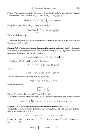
Proof. This result is essentially the change-of-variable formula for integrals. Let f denote
a bounded real-valued function on Y 0 . Then, since f (Y) = f (g(X)),

E[ f (Y)] = E[ f (g(X))] = f (g(x))p X (x) dx.
X 0
Using the change-of-variable y = g(x), we have that

∂h(y)
E[ f (Y)] = f (y)p X (h(y)) dy.
∂y
Y 0
The result follows.
Note that the condition that the Jacobian of g is nonzero is identical to the condition that
the Jacobian of h is finite.

Example 7.5 (Functions of standard exponential random variables). Let X 1 , X 2 denote
independent, standard exponential random variables so that X = (X 1 , X 2 ) has an absolutely
continuous distribution with density function
+ 2
p X (x 1 , x 2 ) = exp{−(x 1 + x 2 )}, (x 1 , x 2 ) ∈ (R ) .
√ √
Let Y 1 = (X 1 X 2 ) and Y 2 = (X 1 /X 2 ). Hence,
Y = (Y 1 , Y 2 ) = g(X) = (g 1 (X), g 2 (X))

where
√ √
g 1 (x) = (x 1 x 2 ) and g 2 (x) = (x 1 /x 2 ).

The inverse function is given by h = (h 1 , h 2 ) where
h 1 (y) = y 1 y 2 and h 2 (y) = y 1 /y 2
which has Jacobian

2y 1
∂h(y)
= .
∂y y 2

+ 2
The set X 0 may be taken to be (R ) and g(X 0 ) = X 0 .
It follows that the distribution of (Y 1 , Y 2 )is absolutely continuous with density function
2y 1
p Y (y 1 , y 2 ) = exp{−y 1 (1/y 2 + y 2 )}, y 1 > 0, y 2 > 0.
y 2
Example 7.6 (Products of independent uniform random variables). Let X 1 , X 2 ,..., X n
denote independent, identically distributed random variables, each with a uniform distribu-
tion on the interval (0, 1). Let

Y 1 = X 1 , Y 2 = X 1 X 2 ,. . . , Y n = X 1 X 2 ··· X n .
Letting X = (X 1 ,..., X n ) and Y = (Y 1 ,..., Y n )wehave Y = g(X) where g =
(g 1 ,..., g n ) with

j

g j (x) = x i , x = (x 1 ,..., x n ).
i=1