Page 219 - Elements of Distribution Theory

P1: JZX
052184472Xc07 CUNY148/Severini May 24, 2005 3:59

7.3 Functions of a Random Vector 205

Then

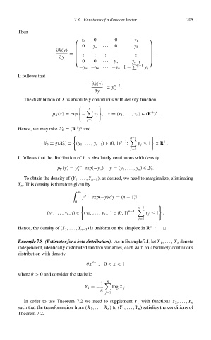
 0 0 
y n ··· y 1
 0 y n ··· 0 y 2
∂h(y)  . . . . . 

=  . . . . . . . . .  .
 .
∂y 
0 0 ··· y n y n−1
 
n−1
−y n −y n ··· −y n 1 − 1 y j
It follows that

= y .
∂h(y) n−1
n
∂y
The distribution of X is absolutely continuous with density function

n
+ n
p X (x) = exp − x j , x = (x 1 ,..., x n ) ∈ (R ) .
j=1
+ n
Hence, we may take X 0 = (R ) and

n−1

+
Y 0 = g(X 0 ) = (y 1 ,..., y n−1 ) ∈ (0, 1) n−1 : y j ≤ 1 × R .
j=1
It follows that the distribution of Y is absolutely continuous with density
p Y (y) = y n−1 exp(−y n ), y = (y 1 ,..., y n ) ∈ Y 0 .
n
To obtain the density of (Y 1 ,..., Y n−1 ), as desired, we need to marginalize, eliminating
Y n . This density is therefore given by
∞

y n−1 exp(−y) dy = (n − 1)!,
0

n−1

(y 1 ,..., y n−1 ) ∈ (y 1 ,..., y n−1 ) ∈ (0, 1) n−1 : y j ≤ 1 .
j=1
Hence, the density of (Y 1 ,..., Y n−1 )is uniform on the simplex in R n−1 .

Example 7.8 (Estimator for a beta distribution). As in Example 7.1, let X 1 ,..., X n denote
independent, identically distributed random variables, each with an absolutely continuous
distribution with density
θx θ−1 , 0 < x < 1

where θ> 0 and consider the statistic
n
1
Y 1 =− log X j .
n
j=1
In order to use Theorem 7.2 we need to supplement Y 1 with functions Y 2 ,..., Y n
such that the transformation from (X 1 ,..., X n )to(Y 1 ,..., Y n ) satisfies the conditions of
Theorem 7.2.