Page 220 - Elements of Distribution Theory

P1: JZX
052184472Xc07 CUNY148/Severini May 24, 2005 3:59

206 Distribution Theory for Functions of Random Variables

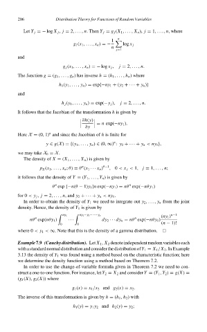
Let Y j =− log X j , j = 2,..., n. Then Y j = g j (X 1 ,..., X n ), j = 1,..., n, where
n
1
g 1 (x 1 ,..., x n ) =− log x j
n
j=1
and

g j (x 1 ,..., x n ) =− log x j , j = 2,..., n.
The function g = (g 1 ,..., g n ) has inverse h = (h 1 ,..., h n ) where
h 1 (y 1 ,..., y n ) = exp{−ny 1 + (y 2 +· · · + y n )}

and
h j (y 1 ,..., y n ) = exp(−y j ), j = 2,..., n.
It follows that the Jacobian of the transformation h is given by

= n exp(−ny 1 ).
∂h(y)
∂y

n
Here X = (0, 1) and since the Jacobian of h is finite for
n
y ∈ g(X) ={(y 1 ,..., y n ) ∈ (0, ∞) : y 2 + ··· + y n < ny 1 },
we may take X 0 = X.
The density of X = (X 1 ,..., X n )isgiven by
n
p X (x 1 ,..., x n ; θ) = θ (x 1 ··· x n ) θ−1 , 0 < x j < 1, j = 1,..., n;
it follows that the density of Y = (Y 1 ,..., Y n )isgiven by
n
n
θ exp {−n(θ − 1)y 1 }n exp(−ny 1 ) = nθ exp(−nθy 1 )
for 0 < y j , j = 2,..., n, and y 2 +· · · + y n < ny 1 .
In order to obtain the density of Y 1 we need to integrate out y 2 ,..., y n from the joint
density. Hence, the density of Y 1 is given by
n−1
ny 1 ny 1 −y 3 −···−y n (ny 1 )
n
n
nθ exp(nθy 1 ) ··· dy 2 ··· dy n = nθ exp(−nθy 1 )
0 0 (n − 1)!
where 0 < y 1 < ∞. Note that this is the density of a gamma distribution.
Example7.9 (Cauchydistribution). Let X 1 , X 2 denoteindependentrandomvariableseach
withastandardnormaldistributionandconsiderthedistributionofY 1 = X 1 /X 2 .InExample
3.13 the density of Y 1 was found using a method based on the characteristic function; here
we determine the density function using a method based on Theorem 7.2.
In order to use the change-of-variable formula given in Theorem 7.2 we need to con-
struct a one-to-one function. For instance, let Y 2 = X 2 and consider Y = (Y 1 , Y 2 ) = g(X) =
(g 1 (X), g 2 (X)) where
g 1 (x) = x 1 /x 2 and g 2 (x) = x 2 .

The inverse of this transformation is given by h = (h 1 , h 2 ) with
h 1 (y) = y 1 y 2 and h 2 (y) = y 2 ;