Page 221 - Elements of Distribution Theory

P1: JZX
052184472Xc07 CUNY148/Severini May 24, 2005 3:59

7.3 Functions of a Random Vector 207

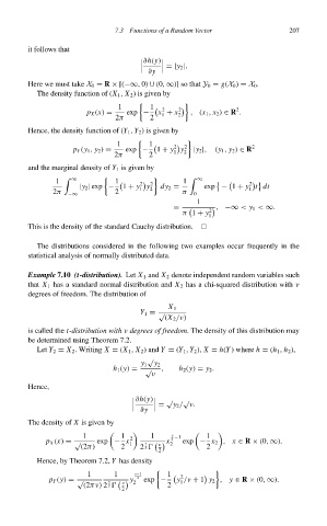
it follows that

=|y 2 |.
∂h(y)

∂y
Here we must take X 0 = R × [(−∞, 0) ∪ (0, ∞)] so that Y 0 = g(X 0 ) = X 0 .
The density function of (X 1 , X 2 )isgiven by
1 1 2 2 2
p X (x) = exp − x + x 2 , (x 1 , x 2 ) ∈ R .
1
2π 2
Hence, the density function of (Y 1 , Y 2 )isgiven by
1 1 2 2 2
p Y (y 1 , y 2 ) = exp − 1 + y y 2 |y 2 |, (y 1 , y 2 ) ∈ R
1
2π 2
and the marginal density of Y 1 is given by
1 ∞ 1 2 2 1 ∞ 2
|y 2 | exp − 1 + y y 2 dy 2 = exp − 1 + y t dt
1
1
2π 2 π 0
−∞
1
= 2 , −∞ < y 1 < ∞.
π 1 + y
1
This is the density of the standard Cauchy distribution.
The distributions considered in the following two examples occur frequently in the
statistical analysis of normally distributed data.

Example 7.10 (t-distribution). Let X 1 and X 2 denote independent random variables such
that X 1 has a standard normal distribution and X 2 has a chi-squared distribution with ν
degrees of freedom. The distribution of

X 1
Y 1 = √
(X 2 /ν)
is called the t-distribution with ν degrees of freedom. The density of this distribution may
be determined using Theorem 7.2.
Let Y 2 = X 2 . Writing X = (X 1 , X 2 ) and Y = (Y 1 , Y 2 ), X = h(Y) where h = (h 1 , h 2 ),
√
y 1 y 2
h 1 (y) = √ , h 2 (y) = y 2 .
ν
Hence,

√ √
∂h(y)
= y 2 / ν.
∂y

The density of X is given by
1 1 2 1 ν −1 1
p X (x) = √ exp − x 1 ν x 2 2 exp − x 2 , x ∈ R × (0, ∞).
ν
(2π) 2 2 2 2
2
Hence, by Theorem 7.2, Y has density
1 1 ν−1 1 2
p Y (y) = √ ν y 2 2 exp − y /ν + 1 y 2 , y ∈ R × (0, ∞).
1
(2πν) 2 2 ν 2
2