Page 346 - Elements of Chemical Reaction Engineering Ebook

Sec. 6.6 The Attainable Region 31 7

0.00014

0.00012

0.00010
C: CSTR8iPFR * 0.00008
A: CSTR
67
B: PFR
2
-
Y
m 0.00006
u
0.00004

0.~00002

0.1DOOI.Xl
0.0 0.2 0.4 0.6 0.8 1 .o
CA (km011m3)

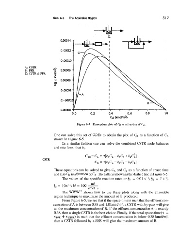
Figure 6-5 Phase plane plots of C, as a function of C, .

One Cim solve this set of ODES to obtain the plot of C, as a function of CA
shown in Figure 6-5.
In a similar fashion one can solve the combined CSTR mole balances
and rate laws, that is,

CSTR

These equations can be solved to give CA and C, as a function of space time
and also CB as a hnction of C,. The latter is shown as the dashed line in Figure 6-5.
The values of the specific reaction rates or kl = 0.01 s-I, k2 = 5 s-',
k3 = 10 S-l, k4 z= 100 -
m3
kmol s
The WWW12 shows how to use these plots along with the attainable
region technique to maximize the amount of B produced.
From Figure 6-5, we see that if the space-time is such that the effluent con-
centration of A is between 0.38 and 1.0 km0Vm3, a CSTR with by-pass will give
us the maximum concentration of B. If the effluent concentration A is exactly
0.38, then a single CSTR is the best choice. Finally, if the total space-time (7: =
+
)
~
~~d T ~ is ~ such that the effluent concentration is below 0.38 kmol/m3,
then a CSTR followed by a PFR will give the maximum amount of B.