Page 477 - Elements of Chemical Reaction Engineering Ebook

448 Steadyetate Nonisothermal Reactor Design Chap. 8

To = Too + AT,, = 58°F + 17°F = 75°F
= 535"R (E8-4.11)
TR = 68°F =t 528"R
The conversion calculated from the energy balance, XEB, for an adiabatic
reaction is found by rearranging Equation (8-52):

(E8-4.6)

Substituting all the known quantities into the mole and energy balances gives us
(403.3 Btu/lb mol. "F)(T - 535)"F
Plot XEB as a = - [ - 36,400 - 7(T - 528)] Btu/lb mol
function of
-
temperature - 403.3(T- 535) (E8-4.12)
36,400 + 7( T - 528)
The conversion calculated from the mole balance, Xm, is found from Equa-
tion (E8-4.5).
(16.96 X 10l2 h-l)(0.1229 h) exp(-32,400/1.987T)
Plot X, as a xMB = 1 + (16.96X 10l2 h-l)(0.1229 h) exp(-32,400/1.987T)
function of
temperature - (2.084 X loi2) exp (- 16,306/T)
-
1 + (2.084 X 10l2) exp (- 16,306/T) (E8-4.13)
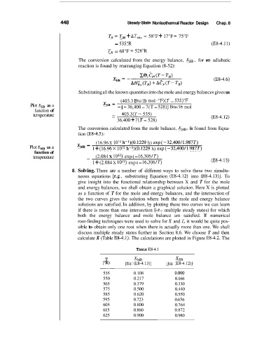
8. Solving. There are a number of different ways to solve these two simulta-
neous equations [e.g., substituting Equation (E8-4.12) into (E8-4.13)]. To
give insight into the functional relationship between X and T for the mole
and energy balances, we shall obtain a graphical solution. Here X is plotted
as a function of T for the mole and energy balances, and the intersection of
the two curves gives the solution where both the mole and energy balance
solutions are satisfied. In addition, by plotting these two curves we can learn
if there is more than one intersection (i.e., multiple steady states) for which
both the energy balance and mole balance are satisfied. If numerical
root-finding techniques were used to solve for X and T, it would be quite pos-
sible to obtain only one root when there is actually more than one. We shall
discuss multiple steady states further in Section 8.6. We choose T and then
calculate X (Table E8-4.1). The calculations are plotted in Figure E8-4.2. The

TABLE E8-4.1

T XMB XEB
(OR) [Eq. (E8-4.13)] [Eq. (E8-4.12)]
-~
535 0.108 O.Oo0
550 0.217 0.166
565 0.379 0.330
575 0.500 0.440
585 0.620 0.550
595 0.723 0.656
605 0.800 0.764
615 0.860 0.872
625 0.900 0.980