Page 210 - Academic Press Encyclopedia of Physical Science and Technology 3rd Chemical Engineering

P1: GAE/LSK P2: FLV Final Pages
Encyclopedia of Physical Science and Technology EN004D-ID159 June 8, 2001 15:47

Crystallization Processes 107

Transforming a mass distribution to a number distri- From Eq. (37), it can be demonstrated that the total num-
bution, or vice versa, requires a relationship between the ber of crystals, the total length, the total area, and the
measured and desired quantities. The mass of a single total volume of crystals, all in a unit of sample volume,
crystal, m crys , is related to crystal size by the volume shape can be evaluated from the zeroth, first, second, and third
factor, k vol (see Eq. (19)): moments of the population density function. Moments of
the population density function also can be used to esti-
3
m crys = ρk vol L (31)
mate number-weighted, length-weighted, area-weighted,
Consequently, the number of crystals on a sieve in the and volume- or mass-weighted quantities. These averages
example, N i , can be estimated by dividing the total mass are calculated from the general expression:
on sieve i by the mass of an average crystal on that sieve. If
¯ m j+1 (38)
the crystals on that sieve are assumed to have a size equal L j+1, j =
m j
to the average of the sieve through which they have passed
¯
and the one on which they are held, L i = (L i−1 + L i )/2, where j = 0foranumber-weightedaverage,1foralength-
then: weighted average, 2 for an area-weighted average, and
3 for a volume- or mass-weighted average.
M i
N i = (32) Crystal size distributions may be characterized usefully
ρk vol L ¯ 3 i (though only partially) by a single crystal size and the
Potassium nitrate crystals have a density of 2.11 × 10 −12 spread of the distribution about that size. For example,
3
g/µm , which allows for the determination of the esti- the dominant crystal size represents the size about which
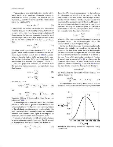
mated crystal numbers on each sieve in Table II. A cumu- the mass in the distribution is clustered. It is defined as
lative number distribution, N(L), and a cumulative num- the size, L D , at which a unimodal mass density function
ber fraction distribution, F(L), can be calculated using is a maximum, as shown in Fig. 11; in other words, the
methods similar to those for calculating M(L) and W(L). dominant crystal size L D is found where dm/dL is zero.
Mass and population densities are estimated from (The data used to construct Fig. 11 are from Table II.) As
the respective cumulative number and cumulative mass the mass density is related to the population density by:
distributions: 3
m = ρk v nL (39)
¯ M i
m(L) = (33) the dominant crystal size can be evaluated from the pop-
L i
ulation density by:
¯ N i
n(L) = (34) d(nL )
3
L i
= 0 at L = L D (40)
dL
So that if L i → 0,
The spread of the mass-density function about the dom-
dM(L) ∞

m(L) = ⇒ M(L) = mdL (35) inant size is the coefficient of variation (c.v.) of the CSD.
dL 0
and
dN(L) ∞
n(L) = ⇒ N(L) = ndL (36)
dL 0
Equations (33) and (34) are used to obtain the last two
columns of Table II.
In the example, all of the results are for the given sam-
ple size of 1 liter and the quantities estimated have units
reflecting that basis. This basis volume is arbitrary, but use
of the calculated quantities requires care in defining this
basis consistently in corresponding mass and population
balances. The volume of clear liquor in the sample is an
alternative, and sometimes more convenient, basis.
Moments of a distribution provide information that can
be used to characterize particulate matter. The jth moment
of the population density function n(L)isdefined as:
∞

j
m j = L n(L) dL (37) FIGURE 11 Mass–density function with single mode showing
0 dominant size.