Page 263 - Academic Press Encyclopedia of Physical Science and Technology 3rd Chemical Engineering

P1: GLM/GLT P2: GLM Final
Encyclopedia of Physical Science and Technology En006G-249 June 27, 2001 14:7

Fluid Dynamics (Chemical Engineering) 55

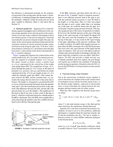
the efficiency is determined primarily by the mechani- If the HGL intersects and drops below the GP, as in
cal precision of the moving parts and the motor’s electri- the area of Fig. 4 marked “region of negative pressure,”
cal efficiency. Centrifugal pumps also depend strongly on there is not sufficient pressure head in the pipe to pro-
the hydraulic conditions inside the pump and are much vide the potential energy necessary to raise the fluid to
more variable in efficiency. More is said about this in the height z at that point. Thus, if a hole were poked
Section VI. into the pipe at such a point, rather than a jet spurting
out of the pipe, air would be drawn into the pipe. In a
d. Hydraulic grade line. Equation (63) is a finite dif- closed pipe a negative gauge pressure develops. This neg-
ference equation and applies only to differences in the var- ative gauge pressure is the source of operation of a siphon.
ious energy quantities at two discrete points in the system. If, however, the absolute pressure in this part of the pipe
It takes no account of any conditions intermediate to these drops to the vapor pressure of the liquid, the liquid will
two reference points. If one were to keep point 1 fixed and boil. This may cause the formation of a vapor bubble at
systematically vary point 2 along the length of the pipe, the the top of the pipe, or it may result in full vapor locking
values of the various heads calculated would represent the of the pipe, depending on the pressure conditions. This
systematic variation of velocity, potential, pressure, pump, is called cavitation. Downhill of the negative pressure re-
and friction head along the pipe route. If all these values gion where the HGL reemerges above the GP, the pressure
were plotted as a function of L, the distance down the pipe rises back above the vapor pressure of the liquid and the
from point 1, a plot similar to that shown schematically in vapor recondenses. This can occur with almost explosive
Fig. 4, would be obtained. violence and can result in physical damage to the pipe. Re-
Figure 4 graphically illustrates the relation between the gions where this cavitation occurs are called “slack flow”
various heads in Eq. (63). For a pipe of constant cross sec- regions. The HGL plot provides a simple and easy way
2
tion, the equation of continuity requires v /2g = 0. to identify potential slack flow regions. In good design,
The pump, located as shown, creates a positive head such regions are avoided by the expedient of introducing
h s = ˆw s /g, represented by the vertical line of this height anotherpumpjustupstreamofthepointwheretheHGLin-
at the pump station (PS). The straight line of slope −h f /L tersects the GP. Details of such procedures are discussed in
drawn through the point (h s , 0) is a locus of all values of Section VI.
potential ( z), pressure ( p/ρg), and friction (h f ) heads
calculated from Eq. (63) for any length of pipe (L). It is 3. Thermal Energy (Heat Transfer)
called the hydraulic grade line (HGL). The vertical dis-
tance between the HGL and the constant value −h s rep- Just as the macroscopic mechanical energy equation is
resents the energy that has been lost to that point due to used to determine the relations between the various forms
friction. The height z designated as ground profile (GP) of mechanical energy and the frictional energy losses, so
is a locus of physical ground elevations along the pipeline the thermal energy equation, expressed in macroscopic
route and is also the actual physical location of the pipe form, is used to determine the relation between the tem-
itself. The difference between the HGL and the GP is the perature and heat transfer rates for a flow system.
pressure head p/ρg at the length L. The significance of When Eq. (46) is applied to the thermal energy terms,
this head is that if one were to poke a hole in the pipe at we obtain
point L,a fluid jet would spurt upward to a height equal to ∂U
˙
˙
the HGL at that point. Thus, the HGL shows graphically at + ρuv · n 1 A 1 + ρuv · n 2 A 2 = Q + F + Q CR ,
∂t
each point along the pipeline route the available pressure
(67)
head to drive the flow through the pipe.
where U is the total internal energy of the fluid and the
other terms have the significance already discussed.
Equation (67) is the basis of practical heat transfer cal-
culations. In order to use it to solve problems, additional
information is required about the total heat transfer rate
˙
Q and the production rate Q . The first is usually ex-
CR
pressed in terms of a heat transfer coefficient analogous
to the friction factor,
˙
Q = U m A s T m , (68)
where U m is an “overall” heat transfer coefficient, which
FIGURE 4 Illustration of hydraulic grade line concept. is usually related to “local” heat transfer coefficients both