Page 267 - Academic Press Encyclopedia of Physical Science and Technology 3rd Chemical Engineering

P1: GLM/GLT P2: GLM Final
Encyclopedia of Physical Science and Technology En006G-249 June 27, 2001 14:7

Fluid Dynamics (Chemical Engineering) 59

1. Newtonian c. Herschel–Bulkley. The pertinent results are
The most important case of this transition for chemical 6464n (2+n)/(1+n) F(ξ 0c , n) 2−n
Re HBc = (2 + n) ,
engineers is the transition from laminar to turbulent flow, (1 + 3n) 2 (1 − ξ 0c ) n
which occurs in straight bounded ducts. In the case of
(116)
Newtonian fluid rheology, this occurs in straight pipes
whenRe = 2100.Asimilarphenomenonoccursinpipesof where ξ 0c is the root of
other cross sections, as well and also for non-Newtonian
(2−n)/n
ξ 0c 1
fluids. However, just as the friction factor relations for
(1 − ξ 0c ) 1+n (1 − ξ 0c ) n
these other cases are more complex than for simple New-
tonian pipe flow, so the criteria for transition to turbu- nHe HB
lence cannot be expressed as a simple critical value of a = 3232(2 + n) (2+n)/(1+n) . (117)
Reynolds number.
He HB is given by Eq. (104) and F(ξ 0c , n) is given by Eq.
All pressure-driven, rectilinear duct flows, whether
(88) evaluated with ξ = ξ 0c .
Newtonian or non-Newtonian, undergo transition to
turbulence when the transition parameter K H of Hanks, d. Casson. The pertinent equations are
defined by
Re CAc = CaG(ξ 0c )/8ξ 0c , (118)
2
ρ|∇v /2|
K H = , (109) where ξ 0c must be determined from the simultaneous so-
|ρg − ∇p|
lution of Eqs. (119) and (120),
achieves a maximum value of 404 at some point in the duct 8 1/2 1/2 3/2
flow. In this equation v is the laminar velocity distribu- 0 = 1 + 2ξ 0c − ξ + 2ξ ¯ ξ 0c − 8ξ 0c ξ ¯
3 0c
tion. In the special limit of Newtonian pipe flow, Eq. (109)
26 1/2 3/2 ¯ 2
¯
reduces the Re c = 2100. For the concentric annulus, it + 3 ξ 0c ξ − 3ξ (119)
reduces to ¯ 2 ¯
6464ξ 0c /Ca = 1 − ξ + 2ξ 0c (1 − ξ)
2
¯ ¯
¯
2
¯
2
Re DC = 808F(σ)/[(1 − ξ + 2λ ln ξ)|ξ − λ /ξ|], 8 1/2 3/2 1/2 1/2 2

− ξ (1 − ξ ¯ ) ξ ¯ − ξ (120)
(110) 3 0c oc
¯
where ξ is the root of and G(ξ 0c ) is given by Eq. (92) evaluated with ξ = ξ 0c .
2
2 2
2
¯
2
2
¯
¯
2
(1 − ξ + 2λ ln ξ)(λ + ξ ) − 2(ξ − λ ) = 0 (111)
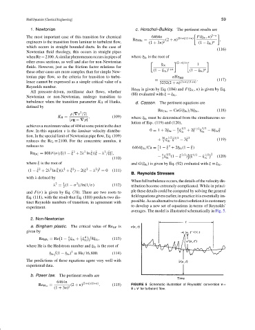
B. Reynolds Stresses
with λ defined by
When full turbulence occurs, the details of the velocity dis-
1
2
2
λ = (1 − σ )/ln(1/σ) (112) tribution become extremely complicated. While in princi-
2
and F(σ) is given by Eq. (78). There are two roots to ple these details could be computed by solving the general
Eq. (111), with the result that Eq. (110) predicts two dis- field equations given earlier, in practice it is essentially im-
tinct Reynolds numbers of transition, in agreement with possible. As an alternative to direct solution it is customary
experiment. to develop a new set of equations in terms of Reynolds’
averages. The model is illustrated schematically in Fig. 5.
2. Non-Newtonian
a. Bingham plastic. The critical value of Re BP is
given by
4 1 4
Re BPc = He 1 − ξ 0c + ξ 8ξ 0c , (113)
3 3 0c
where He is the Hedstrom number and ξ 0c is the root of
3
ξ 0c (1 − ξ 0c ) = He/16,800. (114)
The predictions of these equations agree very well with
experiental data.
b. Power law. The pertinent results are
6464n (2+n)/(1+n)
Re PLc = (2 + n) . (115) FIGURE 5 Schematic illustration of Reynolds’ convention v =
(1 + 3n) 2 ¯ v + v for turbulent flow.