Page 270 - Academic Press Encyclopedia of Physical Science and Technology 3rd Chemical Engineering
P. 270
P1: GLM/GLT  P2: GLM Final
 Encyclopedia of Physical Science and Technology  En006G-249  June 27, 2001  14:7


               62                                                                        Fluid Dynamics (Chemical Engineering)


               VI. APPLICATIONS                                  diagram from them, or one may solve them iteratively
                                                                 for a specific design case. Both methods are illustrated
               A. Friction Factors                               below.
               From a practical point of view the chemical engineer is
                                                                   a. General friction factor plot. The Hedstrom num-
               very often interested in obtaining a relation between the
                                                                 ber is the key design parameter. From its definition in
               overall pressure drop across a pipe, fitting, or piece of pro-
                                                                 Eq. (98) it can be seen that He depends only on the rheo-
               cessing equipment and the bulk or mean velocity of flow
                                                                 logical parameters and the pipe diameter. The rheological
               through it. On occasion the details of the velocity, tem-
                                                                 parameters are obtained from laboratory viscometry data,
               perature, or concentration profile are important, but most
                                                                 and the pipe diameter is at the discretion of the designer
               frequently it is the gross pressure drop-flow rate behavior
                                                                 to specify. Thus, its numerical value is discretionary.
               that is important to a chemical engineer.
                                                                   For a given value of He one can compute a complete
                 This is generally obtained by use of the integrated form
                                                                  f –Re curve as follows:

               of the mechanical energy equation with the frictional en-
               ergy loss calculated by Eq. (65). Thus, the basic problem
               facing a design engineer is how to obtain numerical values  1. Compute Re BPc from Eqs. (113) and (114).
               for the friction factor f .                       2. Using ξ 0c in Eq. (149) compute R ∗ BPc .
                 For Newtonian fluids this problem is solved empiri-  3. For Re BP < Re BPc compute f from Eq. (97).

               cally by the introduction of the Moody diagram (Fig. 3).  4. For Re BP > Re BPc choose a sequence of values of
               In the case of non-Newtonian fluids, however, this is not  R ∗ BP  > R ∗ BPc .
                                                                                        ∗
               appropriate and alternative, semi-theoretical formulations  5. For each such value of R BP  compute ξ 0 from
               must be developed. The theoretical laminar flow equations  Eq. (149) and Re BP from Eqs. (147) and (148).
               for the four rheological models considered here have al-  6. From the computed value of Re BP and the assumed
               ready been presented, as have the modified mixing length  value of R  ∗ BP  compute f from Eq. (138).

               models for turbulent flow of three of these same models.  7. Repeat steps 4–6 as many times as desired and plot

               The latter equations can be integrated to obtain velocity  the pairs of points f ,Re BP so computed to create the
               distributions, which can in turn be integrated to produce  equivalent Moody plot.
               mean velocity–pressure gradient relations. These results
               can then be algebraically rearranged into the desired fric-
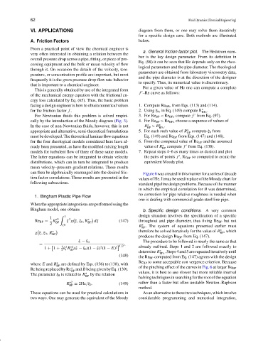
                                                                   Figure6wascreatedinthismannerforaseriesofdecade
               tion factor correlations. These results are presented in the  valuesofHe.ItmaybeusedinplaceoftheMoodychartfor
               following subsections.                            standard pipeline design problems. Because of the manner
                                                                 in which the empirical correlation for B was determined,
                                                                 no correction for pipe relative roughness is needed when
                 1. Bingham Plastic Pipe Flow
                                                                 one is dealing with commercial grade-steel line pipe.
               When the appropriate integrations are performed using the
               Bingham model, one obtains                          b. Specific design conditions. A very common
                        1  ∗2     1  2                           design situation involves the specification of a specific
                 Re BP =  R BP  ξ g ξ, ξ 0 , R ∗ BP  dξ  (147)   throughout and pipe diameter, thus fixing Re BP but not
                        2     ξ0                                   ∗
                                                                  R . The system of equations presented earlier must
                                                                   BP
                                                                                                       ∗
                         ∗                                       therefore be solved iteratively for the value of R , which
                 g ξ, ξ 0 , R BP                                                                       BP
                                                                 produces the design Re BP from Eq. (147).
                                      ξ − ξ 0                      The procedure to be followed is nearly the same as that
                   =                                       ,
                             1 2  ∗2            2      2   1/2   already outlined. Steps 1 and 2 are followed exactly to
                      1 + 1 + k R (ξ − ξ 0 )(1 − ξ) (1 − E)
                             2 t  BP
                                                                 determine R ∗ BPc . Steps 4 and 5 are repeated iteratively until
                                                        (148)
                                                                 the Re BP computed from Eq. (147) agrees with the design
                                                                 Re BP to some acceptable con vergence criterion. Because
               where E and R  ∗  are defined by Eqs. (136) to (138), with
                           BP
               Re being replaced by Re ∗  and B being given by Eq. (139).  of the pinching effect of the curves in Fig. 6 at larger Re BP
                                  BP                             values, it is best to use slower but more reliable interval
               The parameter ξ 0 is related to R ∗  by the relation
                                         BP
                                                                 halving techniques in searching for the root of the equation
                                R ∗2  = 2He/ξ 0 .       (149)    rather than a faster but often unstable Newton–Raphson
                                 BP
                                                                 method.
               These equations can be used for practical calculations in  As an alternative to these two techniques, which involve
               two ways. One may generate the equivalent of the Moody  considerable programming and numerical integration,

