Page 268 - Academic Press Encyclopedia of Physical Science and Technology 3rd Chemical Engineering

P1: GLM/GLT P2: GLM Final
Encyclopedia of Physical Science and Technology En006G-249 June 27, 2001 14:7

60 Fluid Dynamics (Chemical Engineering)

The actual velocity field fluctuates wildly. Reynolds mod- mean values. Thus, any solution of Eq. (10) for the stress
eled it by a superposition of a Eulerian time mean value ¯ v distribution also becomes a solution of Eq. (124) for the
defined by “turbulent” stress distribution. Howe ver, this small suc-

1 t cess extracts a dear price. No further progress can be made

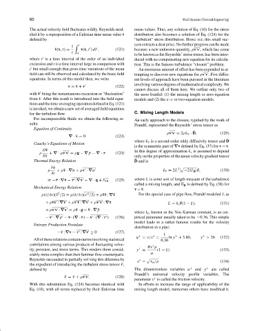
¯ v(x, t) = v(x, t ) dt , (121) because a new unknown quantity, ρv v , which has come
t 0 to be known as the Reynolds’ stress tensor, has been intro-
where t is a time interval of the order of an individual duced with no compensating new equation for its calcula-

excursion and t is a time interval large in comparison with tion. This is the famous turbulence “closure” problem.

t but small enough that gross time variations of the mean An enormous amount of effort has been expended in at-
field can still be observed and calculated by the basic field tempting to discover new equations for ρv v . Five differ-

equations. In terms of this model then, we write ent levels of approach have been pursued in the literature
involvingvariousdegreesofmathematicalcomplexity.We

v = ¯ v + v (122)
cannot discuss all of them here. We outline only two of
with ¯ v being the instantaneous excursion or “fluctuation” the most fruitful: (1) the mixing length or zero-equation

from ¯ v. After this result is introduced into the field equa- models and (2) the κ–ε or two-equation models.
tionsandthetime-averagingoperationdefinedinEq.(121)
is invoked, we obtain a new set of averaged field equations
for the turbulent flow. C. Mixing Length Models
For incompressible fluids we obtain the following re- An early approach to the closure, typified by the work of
sults: Prandtl, represented the Reynolds’ stress tensor as
Equation of Continuity
¯

ρv v = 2ρˆ τ · D, (129)
∇ · ¯ v = 0 (123)
¯
where ˆ τ is a second-order eddy diffusivity tensor and D
Cauchy’s Equations of Motion
is the symmetric part of ∇¯ v defined by Eq. (37) for v = ¯ v.
D¯ v In this degree of approximation ˆ τ is assumed to depend
ρ + ∇ · ρv v = ρg − ∇ ¯ p − ∇ · ¯τ (124)

Dt only on the properties of the mean velocity gradient tensor
¯
Thermal Energy Relation D and is
∂ ¯ u
ρ + ρ¯v · ∇¯ u + ρv · ∇u ˆ τ = 2L 2 −2II ¯ D |δ, (130)

∂t
τ

=− ¯ :∇¯ v − τ :∇v − ∇ · ¯ q + ˙ r CR (125) where L is some sort of length measure of the turbulence
is defined by Eq. (38) for
called a mixing length, and II ¯ D
Mechanical Energy Relation
v = ¯ v.
2
2
ρ(∂/∂t)(¯v /2) + ρ(∂/∂t)(v /2) + ρ¯ v¯ v : ∇¯ v For the special case of pipe flow, Prandtl modeled L as
+ ρ¯ vv : ∇v + ρv ¯ v : ∇v + ρv v : ∇¯ v L = k t R(1 − ξ), (131)

+ ρv v : ∇v = ρ¯ v · g − ¯ v · ∇ ¯ p

where k t , known as the Von Karman constant, is an em-
− v · ∇p − ¯ v · (∇ · ¯τ) − v · (∇ · τ ) (126) pirical parameter usually taken to be ∼0.36. This simple

model leads to a rather famous results for the velocity
Entropy Production Postulate
distribution in a pipe:
− ¯τ :∇v − τ :∇v ≥ 0 (127)

1
+ ∗ + +
u = v/v = ln y + 3.80, y > 26 (132)
All of these relations contains terms involving statistical 0.36
correlations among various products of fluctuating veloc-
Rv ρ
∗
+
ity, pressure, and stress terms. This renders them consid- y = (1 − ξ) (133)
erably more complex than their laminar flow counterparts. µ
Reynolds succeeded in partially sol ving this dilemma by ∗
v = τ w /ρ (134)
the expedient of introducing the turbulent stress tensor ˆτ,
defined by The dimensionless variables u + and y + are called
Prandtl’s universal velocity profile variables. The

ˆ τ = ¯τ + ρv v . (128)
parameter v is called the friction velocity.
∗
With this substitution Eq. (124) becomes identical with In efforts to increase the range of applicability of the
Eq. (10), with all terms replaced by their Eulerian time mixing length model, numerous others have modified it.