Page 272 - Academic Press Encyclopedia of Physical Science and Technology 3rd Chemical Engineering

P1: GLM/GLT P2: GLM Final
Encyclopedia of Physical Science and Technology En006G-249 June 27, 2001 14:7

64 Fluid Dynamics (Chemical Engineering)

∗2
1
n
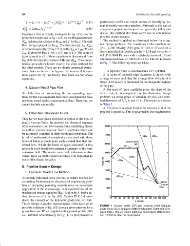
ξ = ξ 0 + (1 − ξ 0 )ζ + R (1 − ξ 0 ) 2/n ∗2 2 (157) particularly useful and simple means of identifying po-
L ζ
8 HB HB
tential trouble spots in a pipeline. Although in this age of

R ∗2 = 2He HB ξ 0 (2−n)/n (158) computers graphic techniques have generally fallen into
HB
disuse, this method still finds active use in commercial
Equation (156) is exactly analogous to Eq. (152) for the
pipeline design practice.
power law model and to Eq. (147) for the Bingham model.
The method is applied as illustrated below for a typ-
R isdefinedinrelationtoRe HB and f byEq.(153),with
∗
HB
∗
Re PL being replaced by Re HB . The function ξ(ξ, ξ 0 , R ) ical design problem. The conditions of the problem are
HB 3
is defined implicitly by Eq. (157), with L ∗ = L HB /R, and Q = 17,280 bbl/day (528 gpm or 0.0333 m /sec) of a
HB
L HB is given by Eqs. (135)–(137) and (141). The value of Newtonian fluid of specific gravity = 1.18 and viscosity =
4.1 cP (0.0041 Pa · sec) with a reliability factor of 0.9 and
ξ 0 to be used in all of these equations is determined from
a terminal end head of 100 ft (30.48 m). The GP is shown
Eq. (158) for specified values of He and R . The compu-
∗
HB
tational procedures follow exactly the steps outlined for in Fig. 7. The following steps are taken:
the other models. There are no simple empirical expres-
sions that can be used to bypass the numerical integra- 1. A pipeline route is selected and a GP is plotted.
tions called for by this theory. One must use the above 2. A series of potential pipe diameters is chosen with
equations. a range of sizes such that the average flow velocity of 6
ft/sec (1.83 m/sec) is bracketed for the design throughput
of the pipe.
4. Casson Model Pipe Flow
3. For each of these candidate pipes the slope of the
As of the time of this writing, the corresponding equa- HGL, −h f /L, is computed. For the illustrative design
tions for the Casson model have been developed but have problem we chose pipes of schedule 40 size with nom-
not been tested against experimental data. Therefore, we inal diameters of 5, 6, 8, and 10 in. The results are shown
cannot include any results. in Table I.
4. The desired residual head at the terminal end of the
pipeline is specified. This is governed by the requirements
5. Other Non-Newtonian Fluids
Thus far we have given exclusive attention to the flow of
purely viscous fluids. In practice the chemical engineer
often encounters non-Newtonian fluids exhibiting elastic
as well as viscous behavior. Such viscoelastic fluids can
be extremely complex in their rheological response. The
le vel of mathematical complexity associated with these
types of fluids is much more sophisticated than that pre-
sented here. Within the limits of space allocated for this
article, it is not feasible to attempt a summary of this very
extensive field. The reader must seek information else-
where. Here we shall content ourselves with fluids that do
not exhibit elastic behavior.
B. Pipeline System Design
1. Hydraulic Grade Line Method
As already indicated, once one has in hand a method for
estimating friction factors, the practical engineering prob-
lem of designing pumping systems rests on systematic
application of the macroscopic or integrated form of the
mechanical energy equation [Eq. (63)], with h f being de-
fined in terms of f by Eq. (65). Section III.C.2.d intro-
duced the concept of the hydraulic grade line, of HGL.
This is simply a graphic representation of the locus of all
FIGURE 7 Ground profile (GP) plot showing initial hydraulic
possible solutions of Eq. (63) along a given pipeline for a
grade lines (HGLs) for pipes of different diameter. Eight- and 10-in.
given flow rate. When coupled with a ground profile (GP) pipes (HGL 8 , HGL 10 ) require additional control point static correc-
as illustrated schematically in Fig. 4, tis plot provides a tion (CPSC) to clear the control point.