Page 271 - Academic Press Encyclopedia of Physical Science and Technology 3rd Chemical Engineering

P1: GLM/GLT P2: GLM Final
Encyclopedia of Physical Science and Technology En006G-249 June 27, 2001 14:7

Fluid Dynamics (Chemical Engineering) 63

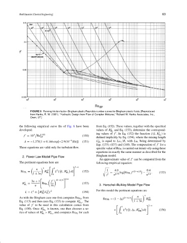
FIGURE 6 Fanning friction factor–Bingham plastic Reynolds number curves for Bingham plastic fluids. [Reproduced
from Hanks, R. W. (1981). “Hydraulic Design from Flow of Complex Mixtures,” Richard W. Hanks Associates, Inc.,
Orem, UT.]

the following empirical curve fits of Fig. 6 have been from Eq. (152). These values, together with the specified
developed: values of R ∗ and Eq. (153), determine the correspond-
PL
ing values of f . In Eq. (152) the function ζ(ξ, R )is

∗
PL
0.193
A

f = 10 Re (150)

BP defined implicitly by Eq. (154), where the mixing length
−5 L ∗ is equal to L PL /R, with L PL being determined by
A =−1.378{1 + 0.146 exp[−2.9(10 )He]} (151) PL

Eqs. (135)–(137) and (140). The computation of f for a
These equations are valid only for turbulent flow. specific value of Re PL is carried out iterati vely using these
equations in exactly the same manner as described for the
Bingham model.
2. Power Law Model Pipe Flow
An approximate value of f can be computed from the

The pertinent equations here are following empirical equation:
2−n
n 1
n ∗2 2
∗
Re PL = R PL ξ ζ ξ, R PL dξ (152) 1 = 4.0 log Re PL f (2−n)/2 − 0.4 . (155)

1 + 3n 0 f n 0.75 n 1.2
(2−n)/2 1/n
3n + 1 f
R ∗ = (153)
PL Re PL
n 16 3. Herschel–Bulkley Model Pipe Flow
∗2
1
n
∗2
ξ = ζ + R L ζ 2 (154) For this model the pertinent equations are
8 PL PL
n

As with the Bingham case one first computes Re PLc from (2−n)/n n ∗2
Re HB = (1 − ξ 0 ) R HB
Eq. (115) and then uses Eq. (153) to compute R ∗ . The 1 + 3n
PLc
value of f to be used in this calculation comes from 2−n

1
Eq. (100). Once R ∗ is known, one then chooses a se- 2 ∗
PLc × ξ ζ ξ, ξ 0 , R HB dξ (156)
ries of values of R ∗ > R ∗ and computes Re PL for each
PL PLc ξ 0