
Page 309 - Academic Press Encyclopedia of Physical Science and Technology 3rd Polymer
P. 309
P1: GQT/MBQ P2: GPJ Final Pages
Encyclopedia of Physical Science and Technology EN014C-660 July 28, 2001 17:14
Rheology of Polymeric Liquids 247
temporary couplings between neighboring chains) begin is imposed on a polymer. The stress remaining in the spec-
to dominate the resistance to flow. For concentrated solu- imen at time t can be determined from a material property
tions and molten polymers, the chain contours are exten- referred to as the stress relaxation modulus G(t), which
sively intermingled, so each chain is surrounded all along for the Rouse model is given by
its length by a mesh of neighboring chain contours. Re-
∞
ρRT
arrangement of macromolecular chains on larger scales G(t) = exp(−t/τ p ), (45)
is restricted because the chain cannot cross through its M p=1
neighbors. The molecular weight between entanglement
where ρ is the density, R is the universal gas constant, T
couplings M e is about one half of M c , i.e., M c ≈ 2M e .In
is the absolute temperature, M is the molecular weight,
the case of polymer solutions, both K and M c in Eq. (44)
and τ p is given by
change if a solvent is added to the polymer.
One can interpret the critical molecular weight M c as a ζb N 2
2
material constant signifying the lower limit of molecular τ p = 6π p k B T , (46)
2 2
weight for which non-Newtonian flow can be observed. It
in which ζ is the segmental friction coefficient, b is the
would then be expected that the onset of non-Newtonian
Kuhn statistical length, N is the number of identical seg-
behavior is strongly dependent on the molecular weight
ments, and k B is the Boltzmann constant. Note that the
and the molecular weight distribution. Above M c , the on-
largest or terminal relaxation time τ 1 for the Rouse chain,
set of non-Newtonian behavior occurs at lower shear rates
i.e., for p = 1 in Eq. (46), is given by
as the molecular weight increases and as the molecular
2
weight distribution broadens. A molecular interpretation (Nζ)(Nb )
of the viscoelastic behavior of polymeric liquids requires τ r = τ 1 = 2 , (47)
6π k B T
different concepts for the two regimes: (a) unentangled
2
regime and (b) entangled regime. where the quantities Nζ and Nb describe the chains as a
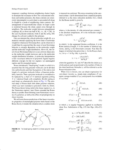
Rouse introduced a “bead-spring” model, in which it is whole and are each proportional to the number of links in
assumed that the long polymer molecule can be divided the chain backbone. Hereafter τ r will be referred to as the
into submolecules and that fluctuations of the end-to-end Rouse relaxation time.
length of a polymer molecule follow a Gaussian proba- When G(t) is known, one can obtain expressions for
0
bility function. Then a polymer molecule is considered to zero-shear viscosity η 0 , steady-state compliance J , dy-
e
be replaced by a chain of N identical segments joining namic storage modulus G (ω), and dynamic loss modulus
N + 1 identical beads with completely flexible spring at G (ω) from
each bead, as schematically shown in Fig. 14. The sem- ∞
inal study of Rouse dealt with dilute polymer solutions, η 0 = G(t) dt, (48)
0
which was later extended to polymeric melts by Zimm.
The Rouse theory being valid in the linear regime (i.e., in 0 1 ∞
J = tG(t) dt, (49)
e
the Newtonian regime), later Zimm extended the Rouse η 0 2 0
theory to predict shear-thinning (non-Newtonian) viscos- ∞
ity of a polymer, as well as the effect of polydispersity on G (ω) = ω G(t) sin ωtdt, (50)
shear viscosity. 0
∞
We will now discuss predictions of the linear viscoelas-
G (ω) = ω G(t) cos ωtdt, (51)
tic properties of unentangled polymer melts based on the 0
Rouse theory. Consider the situation where a sudden strain
in which ω is angular frequency applied in oscillatory
shear flow. Substitution of Eq. (45) into Eqs. (48)–(51)
gives
2
η 0 = (π KρRT/36)M, (52)
0
J = 2M/5ρRT, (53)
e
2 2
∞
ρRT
ω τ p
G (ω) = , (54)
M 1 + ω τ
2 2
p=1 p
∞
ρRT
ωτ p
FIGURE 14 The bead-spring model for a linear polymer mole- G (ω) = . (55)
2 2
M 1 + ω τ
cules. p=1 p