
Page 310 - Academic Press Encyclopedia of Physical Science and Technology 3rd Polymer
P. 310
P1: GQT/MBQ P2: GPJ Final Pages
Encyclopedia of Physical Science and Technology EN014C-660 July 28, 2001 17:14
248 Rheology of Polymeric Liquids
Note that K in Eq. (52) is defined by
2
ζb N 2
K = . (56)
π k B TM 2
2
The Rouse model allows us to determine that stress σ
contributed by the polymer chains by
∞
σ = σ p , (57)
p=2
where σ p denotes the stress contributed by the polymer
chain at the pth mode (p = 1, 2,..., ∞), which can be
evaluated from
∂
1 + τ p σ p = G 0 δ, (58)
∂t
where ∂/∂t is the upper convected derivative, τ p is the
relaxation times defined by Eq. (46), G 0 = ρRT/M, and
δ is the Kronecker delta function.
In steady-state shear flow the Rouse model predicts
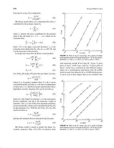
FIGURE 15 Plots of log G versus log ω for a nearly monodis-
∞
ρRT
perse polystyrene with molecular weight of 9 × 10 at various tem-
3
σ = τ p ˙γ, (59)
M peratures: ( ) 120 C, ( ) 130 C, ( ) 140 C, and ( ) 150 C.
◦
◦
◦
◦
p=1
∞
2ρRT
2 2 with molecular weight M less than M c . Figure 15 gives
N 1 = τ ˙γ , (60) plots of log G versus log ω, and Fig. 16 gives plots of
p
M
p=1 log G versus log ω, measured at four different temper-
N 2 = 0. (61) atures for a monodisperse polystyrene with M = 9000,
which is much lower than the M c = 36,000 of polystyrene.
Use of Eq. (46) in Eq. (59) gives the zero-shear viscosity,
It can be seen in these figures that (a) at a constant value
2
ρb ζ N A N 2
η 0 = , (62)
36M
where N A is Avogadro’s number. Since N ∝ M, it can be
concluded from Eq. (62) that η 0 ∝ M and it is independent
of shear rate ˙γ , i.e., the Rouse model cannot predict shear-
dependent viscosity. Equation (62) can be rewritten as
2
ρb ζ 0 N A
0
η 0 = 2 M, (63)
36M
0
where b 0 is the length of monomer, ζ 0 is the monomeric
friction coefficient, and M 0 is the molecular weight of
monomer. The ζ 0 is one of the most important properties
of macromolecules, which can be calculated from Eq. (63)
by measurement of η 0 . With the aid of Eq. (63), Eq. (46)
can be rewritten as
6η 0 M
τ p = , (64)
2 2
π p ρRT
and thus the terminal (Rouse) relaxation time becomes
6η 0 M
τ r = τ 1 = 2 . (65)
π ρRT
FIGURE 16 Plots of lot G versus log ω for a nearly monodis-
The Rouse model is useful to predict the linear vis- perse polystyrene with molecular weight of 9 × 10 at various tem-
3
coelastic properties (Eqs. (52)–(55)) of polymer melts peratures: ( ) 120 C, ( ) 130 C, ( ) 140 C, and ( ) 150 C.
◦
◦
◦
◦