Page 57 - Academic Press Encyclopedia of Physical Science and Technology 3rd Polymer

P1: GQT/LBX P2: GQT/MBQ QC: FYD Final Pages
Encyclopedia of Physical Science and Technology EN008C-602 July 25, 2001 20:31

872 Macromolecules, Structure

¯
The viscosity average molecular weight M v is given by
1/α

¯ α
M v = v i M i
i

1/α
1+α
= N i M N i M i . (36)
i
i i
¯
¯
Note that M v reduces to M w when α = 1. We shall later
see that viscosity measurements made in θ solvents can
be used to provide information about the unperturbed di-
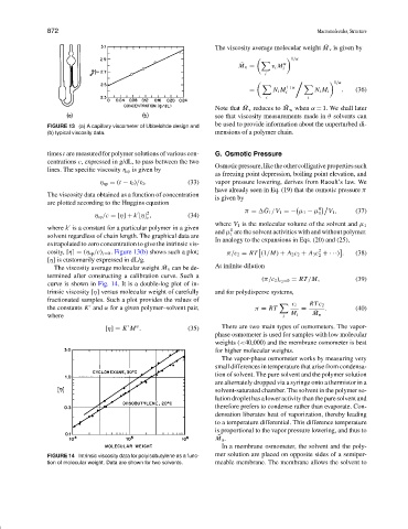
FIGURE 13 (a) A capillary viscometer of Ubbelohde design and
(b) typical viscosity data. mensions of a polymer chain.
times t are measured for polymer solutions of various con- G. Osmotic Pressure
centrations c, expressed in g/dL, to pass between the two
Osmoticpressure,like theothercolligativeproperties such
lines. The specific viscosity η sp is given by
as freezing point depression, boiling point elevation, and
η sp = (t − t 0 )/t 0 . (33) vapor pressure lowering, derives from Raoult’slaw.We
have already seen in Eq. (19) that the osmotic pressure π
The viscosity data obtained as a function of concentration
is given by
are plotted according to the Huggins equation
¯

π = G 1 /V 1 =− µ 1 − µ 0 V 1 , (37)
2

η sp /c = [η] + k [η] , (34) 1
c

where k is a constant for a particular polymer in a given where V 1 is the molecular volume of the solvent and µ 1
0
and µ are the solvent activities with and without polymer.
solvent regardless of chain length. The graphical data are 1
In analogy to the expansions in Eqs. (20) and (25),
extrapolated to zero concentration to give the intrinsic vis-
cosity, [η] = (η sp /c) c =0 . Figure 13(b) shows such a plot; π/c 2 = RT (1/M) + A 2 c 2 + A 3 c + ···) . (38)
2

2
[η] is customarily expressed in dL/g.
¯
The viscosity average molecular weight M v can be de- At infinite dilution
termined after constructing a calibration curve. Such a
(π/c 2 ) c 2 =0 = RT/M, (39)
curve is shown in Fig. 14. It is a double-log plot of in-
trinsic viscosity [η] versus molecular weight of carefully and for polydisperse systems,
fractionated samples. Such a plot provides the values of
c i RT c 2

the constants K and α for a given polymer–solvent pair, π = RT = ¯ . (40)
where i M i M n
α

[η] = K M . (35) There are two main types of osmometers. The vapor-
phase osmometer is used for samples with low molecular
weights (<40,000) and the membrane osmometer is best
for higher molecular weights.
The vapor-phase osmometer works by measuring very
small differences in temperature that arise from condensa-
tion of solvent. The pure solvent and the polymer solution
are alternately dropped via a syringe onto a thermistor in a
solvent-saturated chamber. The solvent in the polymer so-
lution droplet has a lower activity than the pure solvent and
therefore prefers to condense rather than evaporate. Con-
densation liberates heat of vaporization, thereby leading
to a temperature differential. This difference temperature
is proportional to the vapor pressure lowering, and thus to
¯
M n .
In a membrane osmometer, the solvent and the poly-
FIGURE 14 Intrinsic viscosity data for polyisobutylene as a func- mer solution are placed on opposite sides of a semiper-
tion of molecular weight. Data are shown for two solvents. meable membrane. The membrane allows the solvent to