Page 198 - Engineering Digital Design

4.8 MINIMIZATION ALGORITHMS AND APPLICATION 169

ST
ef \ oo 01 ' 11 10
00 f t 1
240 241 1 243 242
ij- ~ TJ
01 J
244 245 I 247 246
11 1 I !/-
252 253 255 254
10 1 1
248 249 251 250 X
Cell 15
T
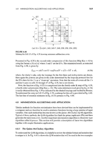
Cell 15 = Zm(241, 243, 245-7, 248, 250, 252, 254, 255)
FIGURE 4.40
Submap for Cell 15 of Fig. 4.39 showing minimum subfunction cover.

Presented in Fig. 4.38 is the second-order compression of this function (Map Key = 4) by
using the format a/b \\cd/ef, where S and T are the EVs. The minimized result, as extracted
from Fig. 4.38, is given by

ZSOP = cdef+aceT+acfS+adT + dS + bf +ab, (4.54)
where, for clarity's sake, only the loopings for the first three and sixth p-terms are shown.
Here again the p-terms are given in the order determined by the loop-out protocol first for
the EVs then for the 1's as a "clean-up" operation. Note that the term ab covers all the 1's
and don't cares in cells 32 through 47 of Fig. 4.38, but is not shown.
Next, the function of Eq. (4.53) is compressed into the fourth-order K-map of Fig. 4.39,
a fourth-order compression (Map Key = 16). The same minimum result given by Eq. (4.54)
is easily obtained from Fig. 4.39 as indicated by the shaded loopings and verified by Boozer.
To understand the entry in Cell 15 of Fig. 4.39, a submap for this cell is provided in Fig. 4.40.
The last line of essential minterms in Eq. (4.53) pertains to Fig. 4.40.

4.8 MINIMIZATION ALGORITHMS AND APPLICATION

Tabular methods for function minimization have been devised that can be implemented by
a computer and can therefore be used to minimize functions having a large number of input
variables. One such method has become known as the Quine-McCluskey (Q-M) algorithm.
Typical of these methods, the Q-M algorithm first finds the prime implicants (Pis) and then
generates the minimum cover. Another important minimization algorithm is a heuristic-type
algorithm called Espresso. This section will provide a description of these two algorithms
together with simple illustrative applications.

4.8.1 The Quine-McCluskey Algorithm
To understand the Q-M algorithm, it is helpful to review the tabular format and notation that
is unique to it. In Fig. 4.41 is shown the Q-M notation that will be used in the two examples