Page 114 - Engineering Electromagnetics, 8th Edition

96 ENGINEERING ELECTROMAGNETICS

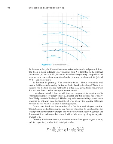
Figure 4.7 See Problem D4.7.
the distance to the point P at which we want to know the electric and potential fields.
The dipole is shown in Figure 4.8a. The distant point P is described by the spherical
coordinates r,θ, and φ = 90 ,in view of the azimuthal symmetry. The positive and
◦
1
negative point charges have separation d and rectangular coordinates (0, 0, d) and
2
1
(0, 0, − d), respectively.
2
So much for the geometry. What would we do next? Should we find the total
electric field intensity by adding the known fields of each point charge? Would it be
easier to find the total potential field first? In either case, having found one, we will
find the other from it before calling the problem solved.
If we choose to find E first, we will have two components to keep track of in
spherical coordinates (symmetry shows E φ is zero), and then the only way to find V
from E is by use of the line integral. This last step includes establishing a suitable zero
reference for potential, since the line integral gives us only the potential difference
between the two points at the ends of the integral path.
On the other hand, the determination of V first is a much simpler problem.
This is because we find the potential as a function of position by simply adding the
scalar potentials from the two charges. The position-dependent vector magnitude and
direction of E are subsequently evaluated with relative ease by taking the negative
gradient of V.
Choosing this simpler method, we let the distances from Q and −Q to P be R 1
and R 2 , respectively, and write the total potential as

Q 1 1 Q R 2 − R 1
V = − =
4π 0 R 1 R 2 4π 0 R 1 R 2