Page 177 - Engineering Electromagnetics, 8th Edition

CHAPTER 6 Capacitance 159

4. Draw in the orthogonal set of field lines. As these are started, they should form
curvilinear squares, but, as they are extended, the condition of orthogonality
should be kept paramount, even though this will result in some rectangles with
ratios other than unity.
5. Look at the regions with poor side ratios and try to see what was wrong with the
first guess of equipotentials. Correct them and repeat the procedure until
reasonable curvilinear squares exist throughout the plot.
6. In regions of low field intensity, there will be large figures, often of five or six
sides. To judge the correctness of the plot in this region, these large units should
be subdivided. The subdivisions should be started back away from the region
needing subdivision, and each time a flux tube is divided in half, the potential
divisions in this region must be divided by the same factor.

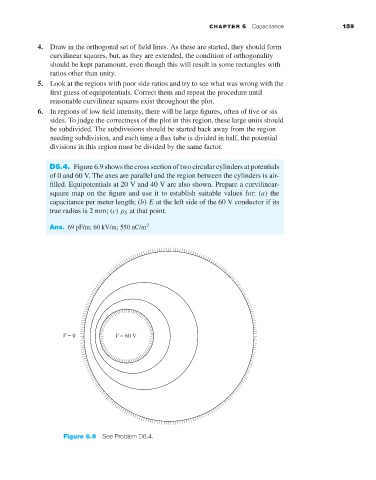
D6.4. Figure 6.9 shows the cross section of two circular cylinders at potentials
of 0 and 60 V. The axes are parallel and the region between the cylinders is air-
filled. Equipotentials at 20 V and 40 V are also shown. Prepare a curvilinear-
square map on the figure and use it to establish suitable values for: (a) the
capacitance per meter length; (b) E at the left side of the 60 V conductor if its
true radius is 2 mm; (c) ρ S at that point.

Ans. 69 pF/m; 60 kV/m; 550 nC/m 2

Figure 6.9 See Problem D6.4.