Page 176 - Engineering Electromagnetics, 8th Edition

158 ENGINEERING ELECTROMAGNETICS

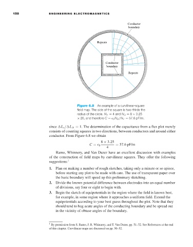
Figure 6.8 An example of a curvilinear-square
field map. The side of the square is two-thirds the
radius of the circle. N V = 4 and N Q = 8 × 3.25
× 26, and therefore C = 0 N Q /N V = 57.6 pF/m.

since L t / L N = 1. The determination of the capacitance from a flux plot merely
consists of counting squares in two directions, between conductors and around either
conductor. From Figure 6.8 we obtain
8 × 3.25
C = 0 = 57.6 pF/m
4
Ramo, Whinnery, and Van Duzer have an excellent discussion with examples
of the construction of field maps by curvilinear squares. They offer the following
suggestions: 1
1. Plan on making a number of rough sketches, taking only a minute or so apiece,
before starting any plot to be made with care. The use of transparent paper over
the basic boundary will speed up this preliminary sketching.
2. Divide the known potential difference between electrodes into an equal number
of divisions, say four or eight to begin with.
3. Begin the sketch of equipotentials in the region where the field is known best,
for example, in some region where it approaches a uniform field. Extend the
equipotentials according to your best guess throughout the plot. Note that they
should tend to hug acute angles of the conducting boundary and be spread out
in the vicinity of obtuse angles of the boundary.

1 By permission from S. Ramo, J. R. Whinnery, and T. Van Duzer, pp. 51–52. See References at the end
of this chapter. Curvilinear maps are discussed on pp. 50–52.