Page 173 - Engineering Electromagnetics, 8th Edition

CHAPTER 6 Capacitance 155

elegant methods, allows fairly quick estimates of capacitance while providing a useful
visualization of the field configuration.
The method, requiring only pencil and paper, is capable of yielding good accu-
racy if used skillfully and patiently. Fair accuracy (5 to 10 percent on a capacitance
determination) may be obtained by a beginner who does no more than follow the
few rules and hints of the art. The method to be described is applicable only to fields
in which no variation exists in the direction normal to the plane of the sketch. The
procedure is based on several facts that we have already demonstrated:

1. A conductor boundary is an equipotential surface.
2. The electric field intensity and electric flux density are both perpendicular to the
equipotential surfaces.
3. E and D are therefore perpendicular to the conductor boundaries and possess
zero tangential values.
4. The lines of electric flux, or streamlines, begin and terminate on charge and
hence, in a charge-free, homogeneous dielectric, begin and terminate only on
the conductor boundaries.
We consider the implications of these statements by drawing the streamlines on
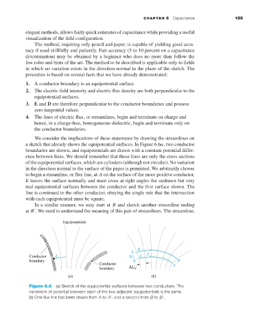
asketch that already shows the equipotential surfaces. In Figure 6.6a,two conductor
boundaries are shown, and equipotentials are drawn with a constant potential differ-
ence between lines. We should remember that these lines are only the cross sections
of the equipotential surfaces, which are cylinders (although not circular). No variation
in the direction normal to the surface of the paper is permitted. We arbitrarily choose
to begin a streamline, or flux line, at A on the surface of the more positive conductor.
It leaves the surface normally and must cross at right angles the undrawn but very
real equipotential surfaces between the conductor and the first surface shown. The
line is continued to the other conductor, obeying the single rule that the intersection
with each equipotential must be square.
In a similar manner, we may start at B and sketch another streamline ending
at B .We need to understand the meaning of this pair of streamlines. The streamline,

Figure 6.6 (a) Sketch of the equipotential surfaces between two conductors. The
increment of potential between each of the two adjacent equipotentials is the same.

(b) One flux line has been drawn from A to A , and a second from B to B .