Page 175 - Engineering Electromagnetics, 8th Edition

CHAPTER 6 Capacitance 157

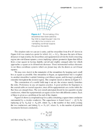
Figure 6.7 The remaining of the
streamlines have been added to
Fig. 6.6b by beginning each new line
normally to the conductor and
maintaining curvilinear squares
throughout the sketch.

The simplest ratio we can use is unity, and the streamline from B to B shown in

Figure 6.6b was started at a point for which L t = L N . Because the ratio of these
distances is kept at unity, the streamlines and equipotentials divide the field-containing
region into curvilinear squares, a term implying a planar geometric figure that differs
from a true square in having slightly curved and slightly unequal sides but which
approaches a square as its dimensions decrease. Those incremental surface elements
in our three coordinate systems which are planar may also be drawn as curvilinear
squares.
We may now sketch in the remainder of the streamlines by keeping each small
box as square as possible. One streamline is begun, an equipotential line is roughed
in, another streamline is added, forming a curvilinear square, and the map is gradually
extended throughout the desired region. The complete sketch is shown in Figure 6.7.
The construction of a useful field map is an art; the science merely furnishes
the rules. Proficiency in any art requires practice. A good problem for beginners is
the coaxial cable or coaxial capacitor, since all the equipotentials are circles while the
flux lines are straight lines. The next sketch attempted should be two parallel circular
conductors, where the equipotentials are again circles but with different centers. Each
of these is given as a problem at the end of the chapter.
Figure 6.8 shows a completed map for a cable containing a square inner conductor
surrounded by a circular conductor. The capacitance is found from C = Q/V 0 by
replacing Q by N Q Q = N Q , where N Q is the number of flux tubes joining
the two conductors, and letting V 0 = N V V, where N V is the number of potential
increments between conductors,

N Q Q
C =
N V V
and then using Eq. (19),

N Q L t N Q
C = = (20)
N V L N N V