Page 472 - Engineering Electromagnetics, 8th Edition

454 ENGINEERING ELECTROMAGNETICS

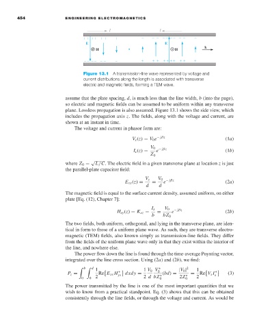
Figure 13.1 A transmission-line wave represented by voltage and
current distributions along the length is associated with transverse
electric and magnetic fields, forming a TEM wave.

assume that the plate spacing, d,is much less than the line width, b (into the page),
so electric and magnetic fields can be assumed to be uniform within any transverse
plane. Lossless propagation is also assumed. Figure 13.1 shows the side view, which
includes the propagation axis z. The fields, along with the voltage and current, are
shown at an instant in time.
The voltage and current in phasor form are:
V s (z) = V 0 e − jβz (1a)

V 0 − jβz
I s (z) = e (1b)
Z 0
√
where Z 0 = L/C. The electric field in a given transverse plane at location z is just
the parallel-plate capacitor field:

V s V 0 − jβz
E sx (z) = = e (2a)
d d
The magnetic field is equal to the surface current density, assumed uniform, on either
plate [Eq. (12), Chapter 7]:

I s V 0 − jβz
H sy (z) = K sz = = e (2b)
b bZ 0
The two fields, both uniform, orthogonal, and lying in the transverse plane, are iden-
tical in form to those of a uniform plane wave. As such, they are transverse electro-
magnetic (TEM) fields, also known simply as transmission-line fields. They differ
from the fields of the uniform plane wave only in that they exist within the interior of
the line, and nowhere else.
The power flow down the line is found through the time-average Poynting vector,
integrated over the line cross section. Using (2a) and (2b), we find:

b d 1 1 V 0 V ∗ |V 0 | 2 1

∗
P z = Re E xs H ys dxdy = 0 (bd) = = Re V s I s ∗ (3)
0 0 2 2 d bZ ∗ 0 2Z 0 ∗ 2
The power transmitted by the line is one of the most important quantities that we
wish to know from a practical standpoint. Eq. (3) shows that this can be obtained
consistently through the line fields, or through the voltage and current. As would be