Page 113 - Essentials of physical chemistry

The First Law of Thermodynamics 75

38.5
4 3 2
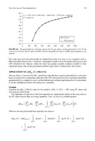
y = –7.137E–12x + 3.109E–08x – 5.035E–05x + 3.722E–02x + 2.658E+01
38
2
R = 9.994E–01
37.5
37
36.5
36
35.5
35
34.5 Series 1
Poly. (series 1)
34
33.5
0 200 400 600 800 1000 1200 1400 1600
FIGURE 4.8 The polynomial fit to the heat capacity for Cl 2 gas where x in the polynomial is T in 8K, the
2
Y-axis is in J=8K mol. The R value of 0.9994 is close to the perfect fit value of 1.0000, which indicates a very
good fit.

Few texts show how the polynomials are obtained but today it is easy to use a program such as
Microsoft Office Excel to fita ‘‘trend line’’ polynomial (Figure 4.8) to the modern data given in the
CRC Handbook [8]. Options within the trend line permit scientific notation extended to four
significant figures (tap on the polynomial and then right click) to obtain results shown here.

APPLICATION TO DH 0 rxn (T > 298.15 K)

Next we show a ‘‘once-in-your-life’’ calculation using the heat capacity polynomials to correct the
heat of a reaction for a temperature other than 298.158K. Obviously this sort of calculation should be
programmed for a computer to carry out the detailed steps in future applications but it is educational
to do the calculations at least once using just a calculator.

Example
0
Calculate the DH rxn (1200 K) value for the reaction 1=2H 2 þ 1=2Cl 2 ! HCl using H values and

f
heat capacity polynomials.
The important concept here is that heat capacities are algebraically subject to the same rules as
0
the H values because they are energy quantities. Thus, we have as a formal equation
f
prod react ð T " prod react #
X X X X
0 0
f,i
DH rxn ¼ n i H n j H f, j þ n i C p,i (T) n j C p, j (T) dT:
i j i j
298:15
When we use the polynomial heat capacities this leads to
ð T ð T ð T ð T
3
DH rxn (T) ¼ DH 0 2 (Dd)T dT
f,298:15 þ (Da)dT þ (Db)TdT þ (Dc)T dT þ
298:15 298:15 298:15 298:15
ð T
4
(De)T dT:
þ
298:15