Page 112 - Essentials of physical chemistry

74 Essentials of Physical Chemistry

4
with the T term the fit is not perfect. We need that higher term to improve the smooth interpolation
4
of the heat capacity for any temperature from 3008K to 15008K. In bygone days, the T term would
have caused an extra hardship in the calculation we are about to do if one were limited to a slide rule
but today students use calculators and personal computers. In fact we are going to do one example,
which could easily be programmed to use a small data library of heat capacity polynomials and H 0
298
values to automate the calculation of DH rxn (T) values in a few milliseconds on a personal computer.
This calculation is the sort of thing that is tedious to do by hand but easy with a computer. However,
a general practice in computer programming is to carry out a check of the method using at least one
pencil-and-paper calculation.

POLYNOMIAL CURVE FITTING
Most students have heard that ‘‘with enough parameters you can draw an elephant,’’ referring to a
danger in curve fitting. Parameterization is useful but can lead to nonsense unless applied with care.
2
The numerical value of the ‘‘coefficient of determination, R ’’ is quoted with the ‘‘trend line’’ fitin
P n 2
2 i (y i f i )
n 2
Excel as a measure of how good the fit is to the data points. Here R 1 P , where
i (y i y)
P n
i y i
y , f i are the values of the trend line function at the respective x i values, and the y i values are
n
the actual data points from the set of (x i , y i ) input. We see that the denominator of the second term is
a positive number as the square of the deviation of the y i points from the average value of ( y) and
represents the range of the y i values, but if the computed f i values of the trend line are all equal to the
2
y i values, the R value will be 1. Note there is a danger here in that a high-order polynomial can
exist, which will pass through every y i point but oscillate wildly between the points. A second
danger is that a tight fit for a set of data points can produce a polynomial, which will diverge greatly
from the data set when a value of x is used outside the range of the data set. The polynomial fit
should only be used for x values within the range of the data set used for the polynomial. Probably
the order of a polynomial fit should not be greater than (n=2) and the best way to fit a curve with a
polynomial is to ‘‘creep up’’ on the best fit by slowly increasing the order of the polynomial as R 2
approaches 1 but make sure the order of the polynomial is less than the number of data points. Here
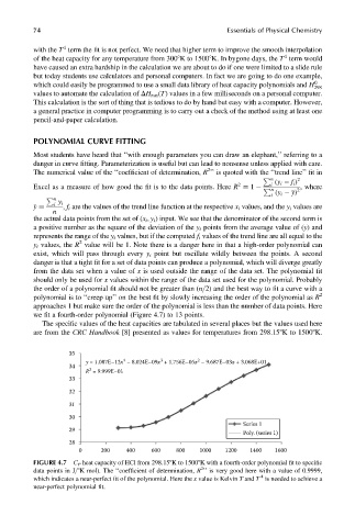
we fit a fourth-order polynomial (Figure 4.7) to 13 points.
The specific values of the heat capacities are tabulated in several places but the values used here
are from the CRC Handbook [8] presented as values for temperatures from 298.158K to 15008K.

35
4 3 2
y = 1.087E–12x – 8.024E–09x + 1.756E–05x – 9.687E–03x + 3.068E+01
34
2
R = 9.999E–01
33
32
31
30
Series 1
29
Poly. (series 1)
28
0 200 400 600 800 1000 1200 1400 1600
FIGURE 4.7 C P heat capacity of HCl from 298.158K to 15008K with a fourth-order polynomial fit to specific
2
data points in J=8K mol). The ‘‘coefficient of determination, R ’’ is very good here with a value of 0.9999,
4
which indicates a near-perfect fit of the polynomial. Here the x value is Kelvin T and T is needed to achieve a
near-perfect polynomial fit.