Page 144 - Essentials of physical chemistry

106 Essentials of Physical Chemistry

p ffiffiffiffiffiffiffiffiffiffiffiffiffiffiffiffiffiffiffiffiffiffiffiffiffiffiffiffiffiffiffiffiffiffiffiffiffiffiffiffiffiffiffiffiffiffiffiffiffiffiffiffiffiffiffiffiffi
ffiffiffiffiffiffiffiffiffiffiffiffiffiffiffiffiffiffi
p 2
2
b 4ac (0:400) 4(0:2271)( 0:03)
b 0:400
; the
2a 2(0:2271)
formula: x ¼ . This leads to x ¼
positive root is x ffi 0:072. Thus, we find at equilibrium: [H 2 ] ¼ 0:300 x ¼ 0:228,
[D 2 ] ¼ 0:100 x ¼ 0:028, [HD] ¼ 2x ¼ 0:144. According to the calculations, almost all of the
D 2 has reacted and been converted to HD noting that H 2 can provide two H atoms.
TEMPERATURE DEPENDENCE OF EQUILIBRIUM CONSTANTS
Sometimes it is possible to shift an equilibrium to increase the yield of a desired product. The key
equation was given above, which shows temperature dependence through the logarithm.
DG 0 298 ¼ RT ln K P and in the example here we have a specific formula:
0
DG 1
298
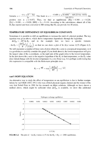
ln K P ¼ , so that we can show a plot of ln (K P ) versus (1=T) (Figure 6.2).
R T(K)
We will encounter a number of these sorts of plots where the x-axis is a reciprocal temperature, so it
is a good idea to carefully consider this graph. If you think about it, the lowest temperature will give
the largest value of the x-coordinate, so the right side of the graph refers to the lowest temperature.
In the plot shown the y-axis is the negative logarithm of the K P at that temperature, so the K P value
does indeed change with the inverse temperature in a very linear way. It is perhaps worth noting that
this expression is compatible with the Boltzmann principle since

0
DG 0 DG 298 E
RT :
K P ¼ e RT ¼ exp ¼ e ðÞ
RT
van’t HOFF EQUATION
An alternative way to study the effect of temperature on an equilibrium is due to further manipu-
lations by van’t Hoff (1852–1911) who was a Dutch physical-organic chemist and the winner of the
very first Nobel Prize in 1901 for his research on dilute solutions. Although we have shown a
method above, which might be sufficient when DG 0 is available, we show this additional
298

Hydrogen exchange equilibrium
0
0 0.0005 0.001 0.0015 0.002 0.0025 0.003 0.0035 0.004
–2

–4
–ln K P –6

–8

–10

–12
1/T (°K)
FIGURE 6.2 The plot of ln (K P ) versus (1=T) for the H 2 þ D 2 ƒ 2HD equilibrium.
ƒ!