Page 163 - Essentials of physical chemistry

Gibbs’ Free Energy and Equilibria 125

qG
i
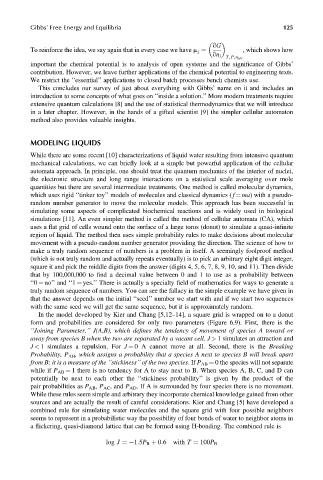
To reinforce the idea, we say again that in every case we have m ¼ , which shows how
qn i
T, P, n j6¼i
important the chemical potential is to analysis of open systems and the significance of Gibbs’
contribution. However, we leave further applications of the chemical potential to engineering texts.
We restrict the ‘‘essential’’ applications to closed batch processes bench chemists use.
This concludes our survey of just about everything with Gibbs’ name on it and includes an
introduction to some concepts of what goes on ‘‘inside a solution.’’ More modern treatments require
extensive quantum calculations [8] and the use of statistical thermodynamics that we will introduce
in a later chapter. However, in the hands of a gifted scientist [9] the simpler cellular automaton
method also provides valuable insights.

MODELING LIQUIDS

While there are some recent [10] characterizations of liquid water resulting from intensive quantum
mechanical calculations, we can briefly look at a simple but powerful application of the cellular
automata approach. In principle, one should treat the quantum mechanics of the interior of nuclei,
the electronic structure and long range interactions on a statistical scale averaging over mole
quantities but there are several intermediate treatments. One method is called molecular dynamics,
which uses rigid ‘‘tinker toy’’ models of molecules and classical dynamics ( f ¼ ma) with a pseudo-
random number generator to move the molecular models. This approach has been successful in
simulating some aspects of complicated biochemical reactions and is widely used in biological
simulations [11]. An even simpler method is called the method of cellular automata (CA), which
uses a flat grid of cells wound onto the surface of a large torus (donut) to simulate a quasi-infinite
region of liquid. The method then uses simple probability rules to make decisions about molecular
movement with a pseudo-random number generator providing the direction. The science of how to
make a truly random sequence of numbers is a problem in itself. A seemingly foolproof method
(which is not truly random and actually repeats eventually) is to pick an arbitrary eight digit integer,
square it and pick the middle digits from the answer (digits 4, 5, 6, 7, 8, 9, 10, and 11). Then divide
that by 100,000,000 to find a decimal value between 0 and 1 to use as a probability between
‘‘0 ¼ no’’ and ‘‘1 ¼ yes.’’ There is actually a specialty field of mathematics for ways to generate a
truly random sequence of numbers. You can see the fallacy in the simple example we have given in
that the answer depends on the initial ‘‘seed’’ number we start with and if we start two sequences
with the same seed we will get the same sequence, but it is approximately random.
In the model developed by Kier and Chang [5,12–14], a square grid is wrapped on to a donut
form and probabilities are considered for only two parameters (Figure 6.9). First, there is the
‘‘Joining Parameter,’’ J(A,B), which defines the tendency of movement of species A toward or
away from species B when the two are separated by a vacant cell. J > 1 simulates an attraction and
J < 1 simulates a repulsion. For J ¼ 0 A cannot move at all. Second, there is the Breaking
Probability, P AB , which assigns a probability that a species A next to species B will break apart
from B; it is a measure of the ‘‘stickiness’’ of the two species.If P AB ¼ 0 the species will not separate
while if P AB ¼ 1 there is no tendency for A to stay next to B. When species A, B, C, and D can
potentially be next to each other the ‘‘stickiness probability’’ is given by the product of the
pair probabilities as P AB , P AC , and P AD . If A is surrounded by four species there is no movement.
While these rules seem simple and arbitrary they incorporate chemical knowledge gained from other
sources and are actually the result of careful considerations. Kier and Chang [5] have developed a
combined rule for simulating water molecules and the square grid with four possible neighbors
seems to represent in a probabilistic way the possibility of four bonds of water to neighbor atoms in
a flickering, quasi-diamond lattice that can be formed using H-bonding. The combined rule is

log J ¼ 1:5P B þ 0:6 with T ¼ 100P B