Page 81 - Essentials of physical chemistry

The Kinetic Molecular Theory of Gases 43

2
perform the same sort of averaging to find the average value of hv i, but we can obtain the same
value by rearranging the average of the kinetic energy to obtain the ‘‘root-mean-square’’ speed,
p ffiffiffiffiffiffiffiffi
2
hv i ¼ v rms . A more useful form is obtained by multiplying both numerator and denominator by
Avogadro’s number, so as to use the molar values of R and the gram molecular weight M.
s ffiffiffiffiffiffiffiffiffiffiffiffiffiffiffiffiffiffiffi
r ffiffiffiffiffiffiffiffi r ffiffiffiffiffiffiffiffiffi
2
mv 3kT m 2 p ffiffiffiffiffiffiffiffi 3kT 3kT(N Av ) 3RT
hv i so then 2 :
2 ¼ 2 ¼ 2 hv i ¼ v rms ¼ m ¼ m(N Av ) ¼ M
An observant student should also note that if the average kinetic energy of particles in three
dimensions is (3kT=2), then one might expect that the kinetic energy is (kT=2) per dimensional
degree of freedom. This is called the law of equipartition of energy and postulates that each degree
of freedom in a given system will lead to an average energy of (kT=2). However, we will eventually
learn that it requires extra explanation in the case of vibrational energy at low temperature.
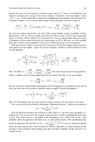
With that exercise in hand, we proceed to the main goal of finding the average speed v instead of
‘‘the square-root of the square.’’ Again, we can use Avogadro’s number to obtain a formula in terms
of mole quantities.

" #
4=2
1 2kT
ð
mv 2
1
2
4p e 2kT (v)v dv 4p r ffiffiffiffiffiffiffiffi r ffiffiffiffiffiffiffiffi
2 m 2 2kT 8kT
0
ð " ffiffiffiffi :
hvi¼ ¼ # ¼ p ¼
mv 2 p p m pm
1 ffiffiffiffi 3=2
4p e 2kT (v) dv 4p 1 . p 2kT
0 2 2 m
r ffiffiffiffiffiffiffiffi r ffiffiffiffiffiffiffiffiffiffiffiffiffiffiffi r ffiffiffiffiffiffiffiffiffi
8kT 8kTN Av 8RT
as the true average speed of the gas particles,
Thus, we obtain hvi¼ ¼ ¼
pm pmN Av pM
which is similar to the root-mean-square speed but not exactly the same, so we can compare
r ffiffiffiffiffiffiffiffiffi r ffiffiffiffiffiffiffiffiffi
8RT p ffiffiffiffiffiffiffiffi 3RT
to 2 :
pM M
hvi¼ hv i ¼ v rms ¼
By now, you should realize that the denominator of the averaging process used above is the same in
each case and refers to the number of particles being averaged. Consider the number N:
ð 1 p ffiffiffiffi 3=2
mv 2 2 p 2pkT
N ¼ 4p e 2kT v dv ¼ 4p :
m 3=2 ¼ m
2 2
0
2kT
Here, 4p will disappear into the factor, but the average numerator will also require a 4p factor.
Thus, we can consider this Maxwell–Boltzmann ‘‘distribution function,’’ which can be written as
m mv 2 2
3=2
f (v) ¼ 4p e 2kT v .
2pkT
You can sketch this function and note that at small values of v, the curve goes up rapidly as a
parabola in v, but at some point, the negative exponent starts to decline asymptotically back down
to zero. Thus, there must be a maximum in the distribution curve, which refers to the ‘‘most
probable’’ speed. In agreement with other texts, we will call this speed a. We can determine this
m mv 2 2
3=2
speed by setting the first derivative of f (v) ¼ 4p e 2kT v to zero to find the maximum
2pkT
where the slope must be zero. Note here that this will be a derivative of a triple product, but the
derivative of the constants will do nothing since they are indeed constants, and the derivative of a
constant is zero.