Page 82 - Essentials of physical chemistry

44 Essentials of Physical Chemistry

df (v) m 3=2 2mv mv 2 2 mv 2
¼ 0 þ 4p e 2kT v þ 2ve 2kT ¼ 0:
dv 2pkT 2kT
The first zero on the right side is due to the derivative of the constants and the other terms are due to
mv 2
the product of v e 2kT . Strictly speaking, we see that this derivative can indeed be zero when v is
2
zero and again when v becomes very large in the negative exponent, but we are interested in the flat

mv 2 m 2
spot at the top of the peak. Thus, we cancel out ve 2kT to leave only v þ 2 ¼ 0, and so we
kT
r ffiffiffiffiffiffiffiffi r ffiffiffiffiffiffiffiffiffiffiffiffiffiffiffi r ffiffiffiffiffiffiffiffiffi
2kT 2kTN Av 2RT
.
m mN Av M
find the most probable speed as a ¼ ¼ ¼
m mv 2 2
3=2
It is difficult to graph f (v) ¼ 4p e 2kT v when you insert the tiny mass ‘‘m’’ and
2pkT
use the high velocities that occur. However, we can consider a simpler function that has the
same variable dependence by using f (x) ¼ e x 2 x 2 as shown in Figure 3.3. The derivative
df 3 x 2 x 2
¼ 2x e þ 2x e ¼ 0 ) x max ¼ 1. We see on the graph that the maximum does indeed
dx
occur at x ¼ 1, but the shape of the curve is asymmetrical and any weighted average using this
distribution will favor higher values of x. By analogy, Figure 3.4 shows that the shape of the
Boltzmann distribution is not symmetric and extends out to the higher speeds. However, the most
important result from the Boltzmann analysis is that now we know the true average speed:
r ffiffiffiffiffiffiffiffiffi r ffiffiffiffiffiffi r ffiffiffiffiffiffiffiffiffi r ffiffiffiffiffiffi
2RT RT 8RT RT
ffi 1:414 , ffi 1:596 , and
V max ¼ hVi¼ V ave ¼
M M pM M
r ffiffiffiffiffiffiffiffiffi r ffiffiffiffiffiffi
3RT RT
ffi 1:732 :
V rms ¼
M M

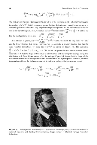
FIGURE 3.3 Ludwig Eduard Boltzmann (1844–1906) was an Austrian physicist, who founded the fields of
statistical mechanics and statistical thermodynamics. (Image courtesy of Chemical Heritage Foundation
Collections.)