Page 57 - Excel Data Analysis

04 537547 Ch03.qxd 3/4/03 11:50 AM Page 43

EVALUATE WORKSHEET DATA 3

You can hide any error messages that may display in a cell
by creating a conditional format definition. To do this,
you use the ISERROR function to create a formula that
checks for an error in the cell. For example, if a formula in
a cell divides by zero, Excel returns the #DIV/0! error
message. To hide any such error messages, select the
range of cells and then click Format ➪ Conditional
Formatting. In the Conditional Formatting dialog box,
click the Formula Is option in the Condition 1 field. In the
next field, type the following definition, replacing A1 with
the first cell in the selected range of cells.
=ISERROR(A1)
By specifying the cell reference of the first cell, Excel
applies the conditional formatting to every cell in the
selected range.
Click the Format button to display the Format Cells dialog
box. In the Font tab, select White as the color and click
OK. The text in any cells containing error messages
displays in white and hides the error messages.

between

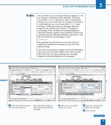
› Click the desired operator Note: If you select Formula Is in ■ Either one or two fields ˇ Type the values for the
from the list of options. step 3, the second list box does display for values. condition in the fields.
not display.
Á Click Format.

CONTINUED

43