Page 337 - Excel for Scientists and Engineers: Numerical Methods

3 14 EXCEL: NUMERICAL METHODS

Nonlinear Least-Squares Curve Fitting
Unlike for linear regression, there are no analytical expressions to obtain the
set of regression coefficients for a fitting function that is nonlinear in its
coefficients. To perform nonlinear regression, we must essentially use trial-and-
error to find the set of coefficients that minimize the sum of squares of
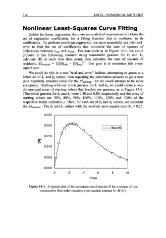
differences between ycalc and yobsd. For data such as in Figure 14-1, we could
proceed in the following manner: using reasonable guesses for kl and k2,
calculate [B] at each time data point, then calculate the sum of squares of
residuals, SSresiduals = C([B]ca~c - [B]e,,t)2. Our goal is to minimize this error-
square sum.
We could do this in a true "trial-and-error" fashion, attempting to guess at a
better set of kl and k2 values, then repeating the calculation process to get a new
(and hopefully smaller) value for the SSresjduals. Or we could attempt to be more
systematic. Starting with our initial guesses for kl and k2, we could create a two-
dimensional array of starting values that bracket our guesses, as in Figure 14-2.
(The initial guesses for kl and k2 were 0.30 and 0.80, respectively and the array of
starting values are 70%, SO%, go%, loo%, 1 lo%, 120% and 130% of the
respective initial estimates.) Then, for each set of kl and k2 values, we calculate
the SSresiduals. The kl and kl values with the smallest error-square sum (kl = 0.27,

0'025 I

0.020

0.01 5

0.01 0

0.005
1

0.000
0 2 4 6 8 10
Time

Figure 14-1. A typical plot of the concentration of species B for a system of two
consecutive first-order reactions (the reaction scheme A+B+C)