
Page 341 - Excel for Scientists and Engineers: Numerical Methods
P. 341
3 18 EXCEL: NUMERICAL METHODS
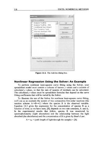
Figure 14-4. The Add-Ins dialog box.
Nonlinear Regression Using the Solver: An Example
To perform nonlinear least-squares curve fitting using the Solver, your
spreadsheet model must contain a column of known y values and a column of
calculated y values, so that the sum of squares of residuals can be calculated.
The calculated y values must be spreadsheet formulas that depend on the curve
fitting coefficients that will be varied by the Solver.
To illustrate the use of the Solver for nonlinear least-squares curve fitting,
we'll use as an example the system of two consecutive first-order reactions (the
reaction scheme A-+B-+C) where the species B is the observed variable.
Equation 14-3 gives the expression for the concentration of species B as a
function of time; as we have seen, [B], depends on two rate constants, kl and k2.
In the experimental results that follow, species B was monitored by
spectrophotometry (light absorption) and the relationship between the light
absorbed (the absorbance) and the concentration of B is given by Beer's Law:
A = E~ x (path length of light through the sample) x [B]