
Page 443 - Excel for Scientists and Engineers: Numerical Methods
P. 443
420 EXCEL: NUMERICAL METHODS
Gaussian Curve. The Gaussian or normal error curve (equation A4-14)
exp[-(x - p)2 /202]
Y= (A4- 14)
OJG
can be used to model UV-visible band shapes, usually in order to deconvolute a
spectrum consisting of two or more overlapping bands. When used for
deconvolution, a simplified form of the Gaussian formula can be used, for
example
A = &axe-[(~-~)~~~l’l (A4- 15)
where A is absorbance, x is the independent variable, either wavelength (e.g.,
nm), or, more commonly, l/wavelength (e.g., cm-’), and in is the value of x at
Amax. The parameters is related to the bandwidth at half-height.
10
8
6
4
2
0
0 2 4 6 8 10
X
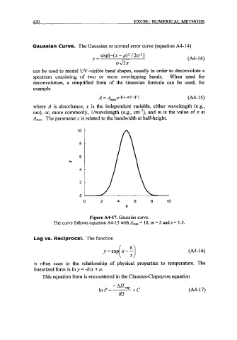
Figure A4-17. Gaussian curve.
The curve follows equation A4-15 with A,, = 10, m = 5 and s = 1.5.
Log vs. Reciprocal. The function
( 3
y=exp a-- (A4-16)
is often seen in the relationship of physical properties to temperature. The
linearized form is In y = -b/x + a.
This equation form is encountered in the Clausius-Clapeyron equation
(A4-17)